Signal vs. Noise, Part 2: Hunter Opens the Klassen Study Again

[Chris_Falter]

@Cornelius_Hunter

there are many more problems with evolution and CD. There are a great many specific examples you can look at. I also like this meta study (Klassen, 1991) of 49 studies. Figure 6 shows how the empirical data consistently do not fit CD:

[I have omitted Hunter’s link to a paywall protected site]

Again, one can always come up with explanations for the empirical data, and that’s fine, but it is important that we’re not talking about anomalies. The data, on the whole, do not fit CD, so you have an enormous parsimony cost with CD

I replied to this in a previous thread. However, I think that I have a better formulation of what Hunter is claiming that I think he will feel is more accurate. In order to try to bring as much light into the conversation as possible, I am deleting my posts in the previous thread, and invite interested readers here instead.

For some reason our friend @Cornelius_Hunter loves to bring up the Klassen 1991 study, even though all but 3 of the 49 datasets demonstrates nested hierarchy at p-value << .025. Here is the diagram I believe that Hunter is referring to:

The consistency index (CI) measures the ratio of feature observations in a taxonomy that would be considered anomalous to a nested hierarchy. The blue region in the graph represents the region where we would expect 95% of the CI calculations to land, given a random assignment of features to taxa. You could refer to the blue region as the null hypothesis regime–i.e., the regime where we can draw no inferences about structural relationships within the taxonomy.

The region above the blue curve is the nested hierarchy regime–i.e., the area where scientists would feel comfortable inferring the existence of a nested hierarchy structure in the taxonomy. Of course, it is useful to ask how confident the inference of a nested hierarchy signal is. Here, the diagram is a great help: the confidence is proportional to the distance from the blue region. The greater the distance, the more confident the inference of nested hierarchy can be.

But we can do better. The statistical significance of any point in Klassen’s scatter plot can be approximated by comparing the vertical distance from the blue region to the vertical size of the blue region at the intersection point. Half of the blue region’s vertical size represents two standard deviations from the mean expected by random assignment of features to taxa. Since the standard deviation is scale-invariant along the Y-axis, we can use the diagram to approximate the number of standard deviations between an observation and the randomness (null hypothesis) mean.

Here is an illustration:

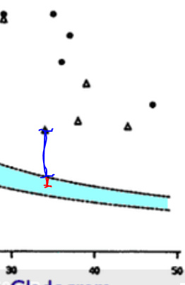
The red line segment represents about 2.0 standard deviations from the randomness/null hypothesis mean. The blue line segment is the distance of a particular observation–the one which is closest to the null hypothesis regime–from the null hypothesis regime. The ratio of the blue segment to the red segment appears to be about 4::1. This means that the observation’s total distance from randomness is about 10.0 standard deviations, i.e., 2.0 SDs along the red line segment and 8.0 SDs along the blue line segment.

Under the null hypothesis, the probability that an observation could lie at a distance of 10.0 SDs is 0.00000000005. Stated another way, the probability that this one taxonomic observation reflects a nested hierarchy rather than randomness is 0.99999999995

Adding even stronger evidence for nested hierarchy in biological taxonomy is the fact that this one observation is one of the weakest in the 49 datasets studied by Klassen. Other observations lie at distances of 20 or even 30 SDs from the randomness mean.

Finally, it is appropriate to take all of the observations as an ensemble. When the vast majority of the observations show the existence of a nested hierarchy with extremely high probability, and only 3 observations with tiny numbers of taxa are in the randomness regime, then the conclusion of nested hierarchy is inescapable.

Unless…

You take Hunter’s approach, which asserts that the existence of any significant amount of noise is evidence against evolution. Hunter stated the following about Klassen 1991 in an old different thread with @Swamidass:

@Cornelius_Hunter

Above about 30, almost all the CI values were less then a half! They ranged from about 0.2-0.4, with random being around 0.15. In other words, the results were far closer to a randomized data set.

Hunter is not arguing over the statistical significance of the hypotheses, he avers. As far as I can tell, he is instead arguing for a Bayesian analysis in which the evolution model products a Consistency Index of 0.8 for all taxonomies, a Design Model predicts a Consistency Index of 0.6 for all taxonomies, and a randomness model predicts a Consistency Index of 0.15 for 30 taxa. (These are the only numbers he has ever supplied in the Signal vs. Noise Part 1 thread, as far as I can tell.) Since the CI scores are closest to the design model, he asserts the design model should win the model selection contest.

Hunter’s Bayesian analysis suffers from four flaws, all of which are fatal to his argument:

(1) The theory of evolution is a stochastic model, so it predicts significant noise.

I have addressed in another thread how the noisiness of stochastic models need not erase a signal, and does not do so in the case of the theory of evolution. I won’t repeat myself.

(2) The mathematical models of evolution predict more noise when more taxa are included in a taxonomic analysis. You can see this by inspecting the blue curve in Klassen’s diagram: increasing the number of taxa decreases the expected Consistency Index for a nested hierarchy.

(3) Per our friend Joshua @Swamidass, computational biologists have quantified the expected CI for taxonomies. The expected value is not the uniform 0.8, but it does conform quite nicely to the observations.

(4) Hunter has been unable to provide any quantitative estimate of the amount of noise predicted by the design model. In the absence of any quantification of predicted noise, it is impossible to predict the CI of the 49 taxonomies under the design model. Since the design model can make no quantified CI predictions, it cannot be included in the Bayesian analysis.

I assert this because I asked Hunter point blank in another thread:

@Chris_Falter

Given robust predictions by a design model, would the design model nevertheless predict noise in real-world observations ? If so, why?

And here was his reply:

@Cornelius_Hunter

these genetic modules that DG [dependency graph] produces are a new construct. They fall out of constructing the DG diagram. So what meaning, if any, do they have? I suspect it will be pretty interesting, and whole new ways of thinking will be opened up. But who knows?

Evidently Hunter does not know.

Hunter cannot make any mathematically-derived statements regarding noise expected under a design model, so it is impossible for the design model to predict how much inconsistency to expect in taxonomies. If the design model cannot quantify how much inconsistency to expect, then the design model cannot make Consistency Index predictions, full stop.

Conclusion

Perhaps, some day, the design model will be sufficiently elaborated in a mathematical way to include it in a Bayesian analysis of Confidence Interval data. If and when that day arrives, who knows the result will be? But that day has not yet arrived. Until it does, it seems premature for Hunter to make any claims based on Klassen (1991) about the supposed inferiority of an evolutionary model to a design model.

Best,
Chris

[Cornelius_Hunter]

@Chris_Falter

You could refer to the blue region as the null hypothesis regime–i.e., the regime where we can draw no inferences about structural relationships within the taxonomy.

Of course you could draw such inferences–there would be no such relationships. That is an inference.

@Chris_Falter

The region above the blue curve is the nested hierarchy regime

Utterly bizarre assertion.

@Chris_Falter

even though all but 3 of the 49 datasets demonstrates nested hierarchy at p-value << .025.

This is a complete misrepresentation, and yet another example of “there are lies, ■■■■ lies, and then there are statistics.” No wonder there has been a concerted move lately against the use of p-values. Some journals have outright banned it.

[GJDS]

@Chris_Falter

The theory of evolution is a stochastic model, so it predicts significant noise.

Hi Chris,

I cannot fathom the meaning of this statement - are you saying ToE can be expressed mathematically as a stochastic formula?

[Chris_Falter]

Good evening, Dr. Hunter.

@Cornelius_Hunter

Chris_Falter: You could refer to the blue region as the null hypothesis regime–i.e., the regime where we can draw no inferences about structural relationships within the taxonomy.

Cornelius_Hunter: Of course you could draw such inferences–there would be no such relationships. That is an inference.

Actually, when a relationship is not found to be statistically significant, that does not mean it does not exist. If the p-value in a two-tailed hypothesis were 0.028, the alternative hypothesis would be rejected in favor of the null hypothesis. The only inference that could be drawn in that case, however, is that the data being studied do not support the alternative hypothesis.

In other words, the absence of statistically significant evidence is not necessarily evidence of absence.

@Cornelius_Hunter

Chris_Falter: The region above the blue curve is the nested hierarchy regime

Cornelius_Hunter: Utterly bizarre assertion.

If you would like to have a discussion, it would help if your entire response to an argument was more than a resort to three-word putdowns.

Perhaps it would have been clearer if you had quoted the entire sentence:

@Chris_Falter

The region above the blue curve is the nested hierarchy regime–i.e., the area where scientists would feel comfortable inferring the existence of a nested hierarchy structure in the taxonomy.

Perhaps I was using jargon from the field of data science, but what I was conveying–or attempting to convey, anyway–is that in the region above the blue curve, the evidence of nested hierarchy reaches statistical significance such that the null hypothesis can be rejected in favor of the alternative hypothesis, which is a tree or nested hierarchy topology.

I trust that this more painstaking definition meets your standards.

@Cornelius_Hunter

This is a complete misrepresentation, and yet another example of “there are lies, ■■■■ lies, and then there are statistics.”

I would be happy to engage with any substance you would like to share, Dr. Hunter. It is rather difficult to engage constructively, however, with a statement like yours.

Grace and peace,
Chris

[Chris_Falter]

Good evening, George. At least by the standards of the eastern US time zone. I think it may not be evening where you are.

@GJDS

are you saying ToE can be expressed mathematically as a stochastic formula?

Yes–if you can consider Turing machines to be mathematical. I consider them to be mathematical, so I answer in the affirmative.

Evolutionary processes can be simulated with software, such as EvolSimulator.

Grace and peace,
Chris

[Cornelius_Hunter]

@Chris_Falter

If you would like to have a discussion, it would help if your entire response to an argument was more than a resort to three-word putdowns.

Contrary to your bizarre statements, low CIs indicate high homoplasy levels.

[GJDS]

Hi Chris,

It is mid-day down here, although I feel as if it were the middle of the night as I work on writing a document of 120,000 words (but I fear it will accelerate to many more).

Thanks for the link _ I have added the remark on my writing as an excuse that enables me to avoid reading or writing additional material. I will say however, that a year or so ago, I had discussed work on gene biology and the reported astronomically difficult task of mathematically providing a direct link with the phenotype. On this basis I would be inclined to treat such simulations with caution/skepticism.

Best wishes

[Chris_Falter]

Good evening, Dr. Hunter,

@Cornelius_Hunter

Contrary to your bizarre statements, low CIs indicate high homoplasy levels.

At the same time, for data sets with numerous taxa, a CI below 0.5 does not erase the phylogenetic signal. As Klassen notes:

A regression through means of random CIs against number of taxa was calculated with a 95% confidence interval. This CI_random is the minimum value that real data sets should exceed to be considered to contain phylogenetic information.

Following Klassen, we can conclude that where CI_random = 0.15 (~35 taxa), a CI of 0.3 carries a strong phylogenetic signal. The vast majority of the 49 data sets in Klassen’s study carry a very strong phylogenetic signal.

You seem to equate the presence of homoplasy with the absence of phylogeny. This is why I entitled the thread, “Signal vs. Noise, Part 2.” According to you, the presence of noise such as homoplasies means there is no phylogenetic signal that would be consistent with evolution. Klassen, however, provides a mathematical definition of the boundary–CI_random–beyond which the phylogenetic signal can be said to disappear. This is why very few if any in the community of biologists are leaping with you. They understand that both signal and noise can exist in the same data set.

Grace and peace,
Chris Falter

[Cornelius_Hunter]

@Chris_Falter

Following Klassen, we can conclude that where CIrandom = 0.15 (~35 taxa), a CI of 0.3 carries a strong phylogenetic signal.

The paper says no such thing. This would be like saying there is “strong” correlation between two variables, because their R^2 value isn’t zero.

@Chris_Falter

You leap to the conclusion that the presence of noise means there is no signal.

No, I said no such thing. You have made a series of untoward and false comments regarding me and the science. When a discussion begins with snide remarks, it usually doesn’t get better (though erasing them was a good move). It is a very predictable pattern. You are trying to twist the data into something that is not there, and the paper into saying something it doesn’t say. This is why people avoid these discussions. If the objective science, and the objective data, are twisted, then there is no basis for discussion.

[T_aquaticus]

@Cornelius_Hunter

The paper says no such thing. This would be like saying there is “strong” correlation between two variables, because their R^2 value isn’t zero.

You are arguing that there isn’t a strong correlation because the r^2 value isn’t 1.00000000. That makes no sense.

You need to define what is and isn’t a strong correlation, and back it up with some statistics instead of your own personal opinion.

[pevaquark (Matthew Pevarnik)]

@Cornelius_Hunter

You are trying to twist the data into something that is not there, and the paper into saying something it doesn’t say.

So would you be able to clearly communicate at least what do you think it says? And in particular what do you think figure 6 says? My first contact with you on this paper was that you really wanted me to look at it as the single figure was very significant to you – in fact so significant that it allows you to easily dismiss all of the ERV evidence for common descent.

[Cornelius_Hunter]

@Chris_Falter

should exceed to be considered to contain phylogenetic information.

You are inferring something that is not intended here. Phylogenetic “information” means very little. In this context, it is synonymous with “not completely random.” They literally scrambled the data to generate a randomized set of data. Phylogenetic “information” simply means that you are outside that random region. That’s it. The data could fit Ewert’s DG model, or some other model. What we do know is that it doesn’t fit CD. The whole point of CI is to measure the number of “moves” required for CD to fit the data. IE, you need to introduce homoplasies. In fact, most of the samples have a CI that is closer to random than to 1!

The use of these data as a proof of CD is an incredible example of the abuse of statistics, and how bad p testing has become.

The fact that evolutionists not only have no problem with these data, but even use it as a proof of CD, is not a success story for CD and evolution. It is another example of how unscientific evolution is. Josh Swamidass has admitted that these data do no harm to evolution and CD. Of course, that has been well known for years, but his admission helps to make that clear. Good for Josh to admit that.

There is a great temptation to avoid falsification and say “my theory can explain that,” in response to any observation. But this is like a drug, as while it feels good, it is corrosive to the theory.

This tendency happens in science, and it empties the theory of any meaning, and makes the theory unfalsifiable. In Bayesian terms, it reduces the probability of the theory because the prior conditional goes down. In model selection terms, the theory has way too many additional terms and is “overfitting.”

Evolution has gone down this road, and is thoroughly addicted to this drug. The literature is loaded with a practically endless sequence special explanations. For CD and phylogenies, practically anything can be explained. You can have extremely rapid evolution or stasis; you can have anagenesis or cladogenesis; you can have the same design appearing repeatedly out of nowhere, any number of times, sporadically in the tree; you can have elaborate designs just disappearing at any time or place in a tree.

The biological world is absolutely loaded with data that do not fit CD. The data do not form a tree. But with all of these add-on explanatory mechanisms, inevitably everything can be explained. In this case, homoplasies can be introduced anywhere, anytime, with no cost to the theory. Unbelievable.

[T_aquaticus]

@Cornelius_Hunter

The data could fit Ewert’s DG model, or some other model.

As we have already seen, Ewert’s model can’t model sequence data. If there is another model you have in mind, now would be the time to bring it forward.

@Cornelius_Hunter

What we do know is that it doesn’t fit CD.

Umm, yes it does:

“Under the null hypothesis, the probability that an observation could lie at a distance of 10.0 SDs is 0.00000000005. Stated another way, the probability that this one taxonomic observation reflects a nested hierarchy rather than randomness is 0.99999999995”-- @Chris_Falter

[Cornelius_Hunter]

@T_aquaticus

You are arguing that there isn’t a strong correlation because the r^2 value isn’t 1.00000000.

No, that is false. Trying to be polite, but you are putting words in my mouth.

[glipsnort (Steve Schaffner)]

@Cornelius_Hunter

The paper says no such thing. This would be like saying there is “strong” correlation between two variables, because their R^2 value isn’t zero.

No, it’s like saying that there is strong evidence for a relationship between two variables even though their R^2 value is 0.5.

[Cornelius_Hunter]

@T_aquaticus

Umm, yes it does:

“Under the null hypothesis, the probability that an observation could lie at a distance of 10.0 SDs is 0.00000000005. Stated another way, the probability that this one taxonomic observation reflects a nested hierarchy rather than randomness is 0.99999999995”-- @Chris_Falter

Well, hey, I tried.

[T_aquaticus]

@Cornelius_Hunter

No, that is false. Trying to be polite, but you are putting words in my mouth.

Then you need to define what r^2 values still allow for a strong correlation across all of these taxa, and back up your analysis with statistics.

[T_aquaticus]

@Cornelius_Hunter

Well, hey, I tried.

You don’t think a p value of 0.00000000005 is good?

[Cornelius_Hunter]

@glipsnort

No, it’s like saying that there is strong evidence for a relationship between two variables even though their R^2 value is 0.5

Arg. Where’s that emoji for head banging against wall.

First, R^2 of .5 is terrible, and normally would be quickly discarded in model selection. Second, to continue the analogy, this is nowhere close even to a lousy R^2 of .5. We’re talking about a CI of 0.3 at ~35 taxa!

Random is ~.15. That’s garbage! And that was optimistic, there are worse samples than that!

Now where’s that emoji?

[pevaquark (Matthew Pevarnik)]

@Cornelius_Hunter

We’re talking about a CI of 0.3 at ~35 taxa!

Random is ~.15. That’s garbage!

Is it? What CI values one should/could get at 35 taxa?

Here’s a tree from a random paper with a CI=0.58 and 31 taxa. Is this garbage too?
https://academic.oup.com/zoolinnean/article/154/3/494/2614026