Nested Clades, The Consistency Index, and Affirming the Consequent

One of the strongest pieces of evidence for evolution is the ‘perfectly nested clade’. This means, when we build a hypothetical evolutionary tree for a dataset of organisms, the organisms more closely match other organisms on their branch of the tree than elsewhere.

The question is, do we see this on real world data? When we have a collection of DNA sequences from different organisms, and try to build a tree, does the tree exhibit this ‘perfectly nested clade’ property? How do we measure such a match?

The measurement of how well the dataset matches the tree is called the phylogenetic signal.
One of the most popular metrics for measuring phylogenetic signal is called the consistency index.

It is very popular partly because of its simplicity. Say we have a dataset of 3 organisms, each organism having 4 genes, and the genes are drawn from a pool of 8 unique genes. We start by counting the total number of unique genes in our dataset, which is 8. We call this number R.

Next, we look at the ancestors of our tree. Let’s say the tree has 2 ancestors. Each ancestor has its own collection of genes. For each node in our tree, whether leaf or ancestor, we subtract from its genes all the genes in its ancestry, leaving only the genes that have never appeared before in the node’s evolutionary history. This subtraction process leaves us with a collection of delta scores, which we then sum together to get the tree length, denoted by L.

Our consistency index is simply c = R/L. The intuition behind the index is that if genes emerge only along a path through the tree, and don’t pop up randomly along other paths, then c will be close to 1. On the other hand, if genes are popping up willy nilly in the tree, then c will be close to 0.

However, c only gets us half way to the phylogenetic signal. We also need an idea what c values to expect under the willy nilly (random) scenario. When we have a good idea of what a randm c value looks like, then we can place a statistical bound on c value that we can say are non random. When c passes this non-random threshold, at that point we say the dataset possesses phylogenetic signal.

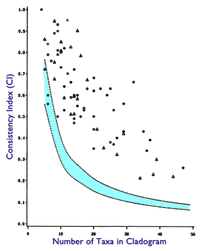
The much lauded example of using the consistency index to measure phylogenetic signal objectively is the Klassen 1991 paper, which has a nice graph pasted below. This paper is held up by the Talk Origins website as very rigorously establishing that species follow the ‘nested clade’ structure much, much better than expected due to randomness. You can see the writeup here.

Seventy-five independent studies from different researchers, on different organisms and genes, with high values of CI (P < 0.01) is an incredible confirmation with an astronomical degree of combined statistical significance (P << 10-300, Bailey and Gribskov 1998; Fisher 1990). If the reverse were true—if studies such as this gave statistically significant values of CI (i.e. cladistic hierarchical structure) which were lower than that expected from random data—common descent would have been firmly falsified.

And here is the plot of the CI index of the 75 different studies compared to the random CI cutoff. As you can see, most of the studies are well above the random CI cutoff, which according to the theory means all these datasets follow the ‘perfectly nested clade’.

Screen Shot 2020-09-04 at 10.35.50 PM

Can we infer evolution from such great statistical significance? Note, the write up claims the converse would falsify evolution, which is indeed true. However, all this statistical significance does not itself verify evolution. Let’s look at the implication being argued:

  1. common descent → nested clades

And let’s look at what we observe:

  1. nested clades

However, we cannot go from 1 and 2 to prove common descent, as this is the fallacy of affirming the consequent. All we can hope to prove with nested clades is apply modus tollens:

  1. not nested clades → not common descent

Thus, nested clades is not evidence of common descent, nor evolution.

As a quick and simple counter example, let’s see a situation where a perfect CI score of 1 is compatible with zero phylogenetic structure (i.e. no tree).

Here we have 3 organisms with 5 genes each (letters are genes):

  1. ABCDE
  2. FGHIJK
  3. LMNOP

Let’s calculate R. Since there are 3 organisms with 5 genes each, then R=3*5=15.

Alright, can we build a tree for this dataset? None of the organisms have any genes in common, so the only tree we can build is a star, where all the organisms have a single ancestor, and this ancestor has zero genes.

What is the length L of the star? Since the delta scores are precisely the gene counts for each organism, then L=3*5=15.

Now, let’s calculate the c value for our scenario. Since c=R/L, then in this case c=15/15=1.0. A perfect consistency index score!

Additionally, even for such a small number of taxa the c score of 1.0 is well above the random cutoff threshold. Or, if it were not, then we can easily extend our scenario to have whatever arbitrary number of taxa required, each with its own unique set of genes, and the score will continue to be 1.0, well above the random cutoff threshold.

So, here we have a scenario that can be repeated to any desired level of statistical significance, which achieves a perfect c score with absolutely no phylogenetic structure!

This is why we cannot invert the implication:

common descent → nested clades

to be:

nested clades → common descent

since it is trivial to come up with a counter example where this is not the case.

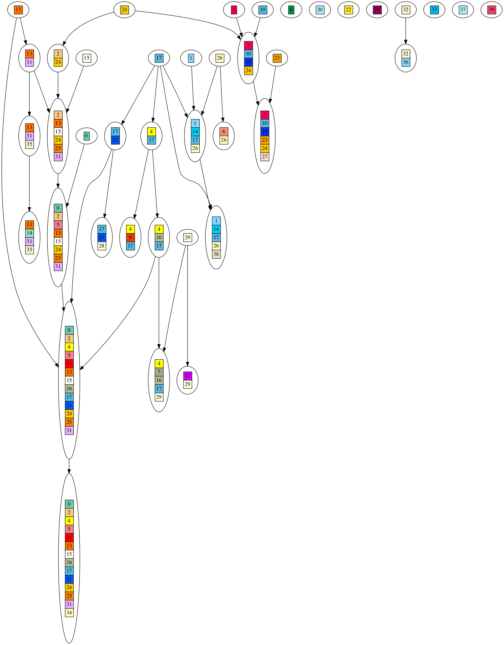
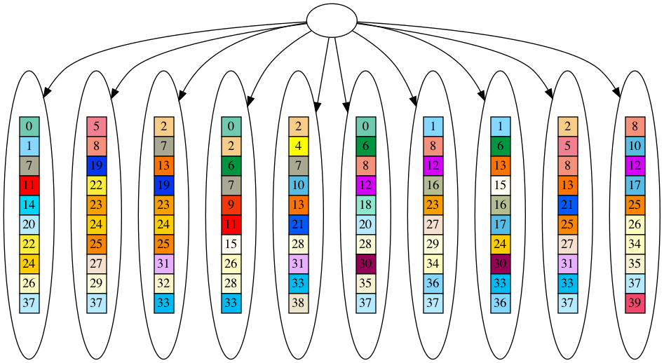
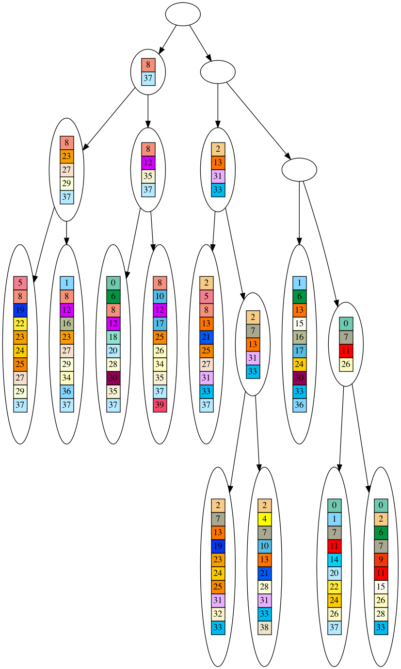
It is also easy to come up with more sophisticated counter examples, such as directed acyclic graphs or randomly generated taxa, but this serves to illustrate the point: ‘perfectly nested clades’ is not evidence for common descent, especially not as presented in the Talk Origins article.


If you want to see more complex scenarios that also easily exceed the random CI cutoff, as well as exceeding all the values in the plot, without evolution, see the source code simulation here. You can run it in your browser and reproduce my results!

https://repl.it/talk/share/The-Phylogenetic-Signal-Fallacy/52293

You can see pictoral examples of the more complex scenarios created by the simulation here: Fallacy of the Phylogenetic Signal? Part 2 - #148 by EricMH

From the Klassen 1991 paper:

Despite its many detractors, the CI remains the most widely used measure of homoplasy and of confidence an investigator might place in a given data set. Its popularity stems from both its simple calculation and its intuitive appeal. It is likely that the CI will continue to be used by phylogenetic systematists as a convenient tool for evaluating data sets and their resulting cladograms.

Definition of CI from the original Kluge 1969 paper:

In the following passages, OTU is “Operational Taxonomic Units”, which the same as the leaf of an evolutionary tree in this discussion.

We use the following conventions: X(A,i) denotes the state of character i for OTU A, and the difference, D(A,B), between OTU A and OTU B is defined to be

D(A,B) = Sum over i: |X(A,i)-X(B,i)|. (1)

The objective of the Wagner method is to form a network, or tree, by connecting all original OTUs and realize in the process a minimum number of changes (“steps” in the sense of Camin and Sokal, 1965) on the tree. This is a network of minimum length in the space in which “length” is defined a certain way.

The connection between OTU A and its most recent ancestor we shall call interval A, using the OTU name to index the interval. The difference, as defined in equation (1), between OTU A and its most recent ancestor, will be called the length of interval A. The length of the tree is the sum of the lengths of all intervals of the tree. The tree of minimum length is defined to be most parsimonious.

We now define the index of consistency, c. The range, r, of character i, r(i), is defined as the difference between the numerically largest and numerically smallest states of the character. The size, R, of the data is defined as

R = Sum over i: r(i)

Letting L stand for the length of the tree, we define the index of consistency of a tree to a set of data as c = R/L, where R, L, and the tree have been computed on the set of data for which c is specified. The value of c lies between 0 and 1. It is 1 if there is no convergence on the tree, and tends to 0 as the amount of convergence on the tree increases. Since c is monotone decreasing on L, c is maximal over trees for a set of data on the most parsimonious tree.

Applying this to my simulation, where I have binary genes that are either present or not present, then the largest and smallest values for each gene are 1 and 0 respectively. Thus, r(i) for each gene is 1-0=1.

So, to calculate R for my scenario, I just count the number of unique genes.

The L for my scenario is the same as the sum of delta scores, where each delta is the set difference between a node and all its ancestors.

@T_aquaticus and @Chris_Falter I would be interested in your thoughts once you have a few minutes to spare. No rush, just making sure you saw this and the thread doesn’t die before you get a chance to respond. I think I’ve been able to show the phylogenetic signal example you rely on is not indicative of evolution, at least the version posted on Talk Origins, and would be interested to know if/where you think I’ve gone wrong.

1 Like

Hi Eric -

I greatly appreciate your interest in getting feedback. While I can occasionally spend a few minutes of reflection or writing about a topic on the forum, the press of my work and M.S. studies prevent me from giving your thought-provoking proposal the attention it deserves.

More scientists with phylogenetics qualifications hang out at Peaceful Science, I believe, so you might try there.

Peace,
Chris

1 Like

Here’s another fun counter example.

Let’s say we have just a single gene. So R always equals 1.

We have a model of evolution where each branch that gene is added once to the descendents. Thus, for each branch we increase the length of the tree by 2N, where N is the number of leaves. By simple arithmetic, this means L=2N-1.

Since c=R/L, then in this scenario c=1/(2N-1). Thus, as N tends towards infinity, then c goes to zero.

As a result, in this case we have a perfectly branching evolutionary process creating the children, yet c=0, which indicates absolutely no phylogenetic structure.

Would you say that the scientific method itself affirms the consequent?

Now that is a complicated question. I would say that to the extent it does, it is not very good science.

The claim is nested clades are more probable on CA. Not that it “proves” CA. If nested clades were the only evidence for CA I probably wouldn’t accept it. But it’s a cumulative case. Many lines of evidence from independent areas of study all come to the same conclusion. The chances of that happening and that conclusion not being true is unlikely. No affirming the consequent here.

http://educ.jmu.edu/~omearawm/deduction.html

2 Likes

Then what is hypothesis testing? A hypothesis states that if you make specific observations then the hypothesis is supported. This is how science works.

More to the point, using nested hierarchies to test the hypothesis of common descent is completely scientific. From our first hand knowledge of genetics, inheritance, and population genetics we know that these processes produce a nested hierarchy. We can then hypothesize that if these mechanisms were active in the past then we should see a nested hierarchy between species, both extinct and extant. How is this not a valid scientific hypothesis?

1 Like

A valid abductive inference is a bit more involved than merely A → B, B, .: A.

Additionally, we have multiple levels of indirection with the Talk Origins article. First we have evolution → nested hierachy. Then we have nested hierachy → some consistency index. Then we observe a certain consistency index. Then we conclude evolution. Way too many hops with little justification to form a valid abductive inference.

As for the consistency index, I’ve derived a closed form solution that allows me to generate a point anywhere on the Talk Origins graph completely without a phylogenetic tree. So, as far as consistency index demonstrating evolution is concerned, it seems pretty valueless.

To whatever extent perfectly nested clades are meant to demonstrate evolution, the Talk Origins article evidence falls short.

I re-read through the Talk Origins section, and it makes a pretty strong claim:

These tests measure the degree of “cladistic hierarchical structure” (also known as the “phylogenetic signal”) in a phylogeny, and phylogenies based upon true genealogical processes give high values of hierarchical structure, whereas subjective phylogenies that have only apparent hierarchical structure (like a phylogeny of cars, for example) give low values

This claim is false. So called ‘subjective phylogenies’, i.e. items placed in a hierarchy that are not produced by a tree like process, can indeed generate very statistically significant phylogenetic signal.

How so? That looks like a completely subjective opinion.

Because the crucial premise of the abductive inference is false. This one:

These tests measure the degree of “cladistic hierarchical structure” (also known as the “phylogenetic signal”) in a phylogeny, and phylogenies based upon true genealogical processes give high values of hierarchical structure, whereas subjective phylogenies that have only apparent hierarchical structure (like a phylogeny of cars, for example) give low values

That’s not what I am seeing. The consistency index for biological species is well above the CI for random data sets, as seen in the opening post.

1 Like

The false claim is this (I previously included the full sentence for context).

whereas subjective phylogenies that have only apparent hierarchical structure (like a phylogeny of cars, for example) give low values

This is false.

See my many examples I’ve given in this forum. Here is the source code again you can run yourself to see DAGs and random datasets generate high CI scores.

From a run I just did:

DAG adjusted CI: 0.8776693649677443
Fake adjusted CI: 0.4103767913550215

“adjusted CI” means I subtracted the CI score for statistical insignificance. Even with this subtraction, the CI score is almost 1 for the DAG, which is the maximum CI score possible. It is also very statistically significant for the randomly generated dataset.

Here’s a visual of such a DAG:

And the corresponding subjective phylogeny derived from that DAG:

All these DAGs are clearly not hierarchical, yet can be fit to a subjective phylogeny with very high statistical significance.

Similarly for a random dataset:

And the corresponding subjective phylogeny:

Which also achieve very statistically significant CI scores.

This directly falsifies the claim:

whereas subjective phylogenies that have only apparent hierarchical structure (like a phylogeny of cars, for example) give low values

As such, the entire article is invalidated.

Then how do you explain the much lower scores for the random data sets in the Klassen paper?

‘random’ has many definitions, and they have a different one than I used.

The point is, my subjective phylogenies achieve CI scores way above the real world datasets, showing ‘statistically significant’ CI scores tell us nothing of significance.

Uh huh. Go figure.

What makes your phylogenies subjective?