The Fallacy of the Phylogenetic Signal? Part 1

I’ve made the argument a couple times on this forum that phylogenetic signal does not tell us whether evolution occurred, since non evolutionary theories will also exhibit a phylogenetic signal. Since the phylogenetic signal cannot discriminate between competing theories, it is not support for evolution.

This is part 1 of my demonstration going over the approach. Part 2 can be found here:

I have written a script to demonstrate this fallacy. The basic idea is it generates datasets a couple different ways, one in line with evolution, and two non evolutionary ways. I then measure the phylogenetic signal in each dataset, and show the non evolutionary datasets actually exhibit stronger phylogenetic signal than the evolutionary dataset.

As a demonstration, here is a dataset generated from an evolutionary tree. The dataset is the leaves of the tree, and I’ve shown the entire tree. It’s a bit long, but this way you can see everything on your screen without scrolling sideways.

It is a very simplistic form of evolution, where each node in the tree represents the generation of a new gene, and no genes are ever lost. If you look closely at the graph, each node in the tree contains little colored boxes with numbers. You can think of each colored box as representing a gene. If two boxes share the same color/number they are the same gene. You can track how the genes accumulate as you trace down the growing tree to the leaves.

Each leaf in the tree you can think of representing a current day species, with its collection of genes picked up during the course of evolution. We cannot time travel backwards to look at the previous nodes in the tree, so we will need to infer these nodes. I will give an example of this inference after the tree picture below (you’ll need to click on the picture to see the full tree, and will need to download it to be able to zoom in on detail).

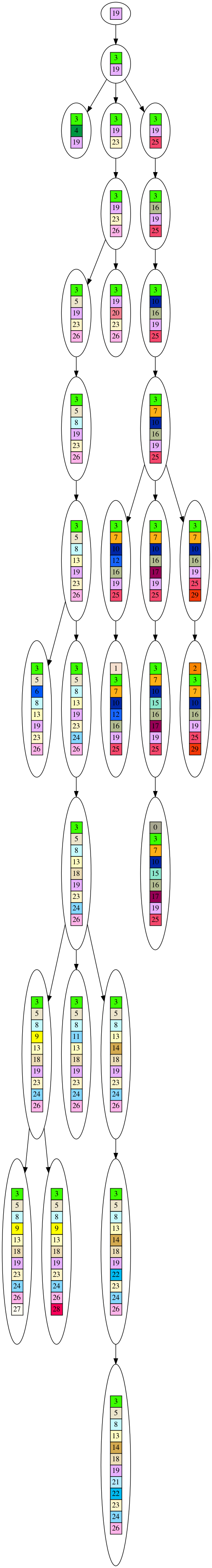
Alright, so now you’ve seen what is meant by evolving a tree with this script, and the kind of dataset it generates. If you look at the leaves of the tree, for instance the leaf with the numbers: “3, 5, 8, 13, 14, 18, 19, 21, 22, 23, 24, 26” is part of the dataset, but the parent node is not part of the dataset. Also, the leaf with the numbers “3, 4, 19” is part of the dataset. Altogether, there are 10 leaves in the dataset.

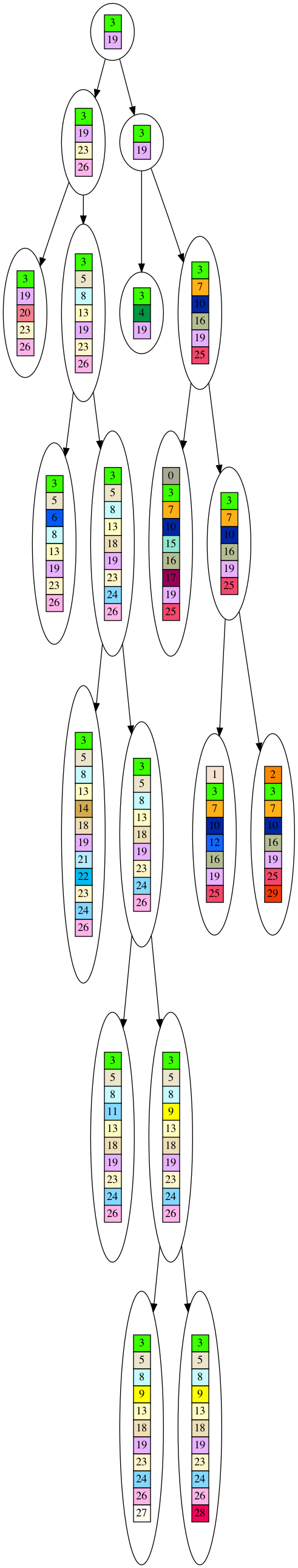
Now that we have the 10 leaf dataset, the question is how do we infer the tree? We cannot travel backwards in time to look at the older nodes, so we have to guess what the ancestors looked like. We will keep the simplistic assumption that genes are never lost, and try to determine what the tree will look like if genes constantly accumulated and were never lost. Here is an example of such a tree inferred froum our 10 leaf dataset (you need to click on the picture to see the full tree, and will need to download it to be able to zoom in on detail).

You’ll notice the tree is much shorter. This is because in the inferred tree nodes are only introduced for speciation events, i.e. branches in the tree. But in the actual evolutionary tree nodes are introduced whenever a new gene appears. If you imagine in your mind squishing the lines of single nodes in the evolutionary tree, you can see how you end up with the inferred tree. Thus, the inferred tree is a faithful, although compressed, reproduction of the evolutionary tree. It looks like our tree inference algorithm is dependable.

But, we cannot rest easy yet. There is a chance, although small, that the observed dataset of 10 leaves was generated by chance of giant leaps instead of through incremental evolution. This is our null hypothesis. To infer a tree, we want to reject the null hypothesis. How do we form and then reject this null hypothesis?

The null hypothesis is that our observed dataset was generated by a star shaped graph instead of a tree. You can see the null hypothesis next. You’ll note there is only one parent node, which contains the few genes common across our 10 leaf dataset.

Finally, our question is, how can we quantitatively reject the null hypothesis in favor of our tree hypothesis? Intutively, if our dataset contained a large number of genes in common, it is not a very big leap from the common pool of genes to each leaf. In which case, we cannot reject the null hypothesis in favor of the tree. We can think of this null hypothesis as a sort of creationist scenario, where a common kind forms the basis of evolution for all the species we see today. I.e. on the ark there was a hippopotamus/horse/cow predecessor, which quickly mutated into the diverse species we see today.

On the other hand, if there are few genes in common across the dataset, then the common kind hypothesis is highly improbable, and our dataset is more likely represented by a large number of small mutations.

To quantify the probability of these two scenarios, we take the gene delta between the parent and child node. For example, if the parent is “1, 2, 3” and the child is “1, 2, 3, 4, 5”, the delta is “4, 5”. The delta is two genes. We then exponentiate 2 to the power of this gene count. In this case, it is 2^2=4. For the entire graph, we sum all the exponentiated deltas to end up with a final score. This score represents the probability inversely, i.e. a very large score indicates a very small probability. Thus, the graph, either tree or star, with the smallest exponentiated delta score is the winning hypothesis. In the case of our example, the tree hypothesis turns out to be the winner.

So, hopefully this explanation clarifies how we infer a tree for a dataset, and how we measure whether the tree is a better fit for the dataset than the null hypothesis, i.e. the phylogenetic signal of the dataset.

Next installment we will measure the phylogenetic signal for datasets generated in a non evolutionary manner.

By showing your work, you give forum participants like me the opportunity to provide feedback. Much appreciated.

My feedback for you is that biologists commonly analyze sequence data rather than gene occurrence data. I can think of a couple of good reasons for this; there are probably many more that I’m not aware of. Allow me to provide some questions that you can, if you choose, leverage in your simulation:

  1. Why do geneticists use sequence data rather than gene occurrence data to steady relationships?
  2. How could this simulation be adapted so that it uses sequence data rather than gene occurrence data?

Peace,
Chris

Yes, this is the same point @T_aquaticus has brought up, that sequence level is more reliable than gene level. I don’t disagree. It is just much more difficult to analyze and simulate. I would like to get there.

Additionally, for the purpose of my argument, I don’t believe going to the sequence level is necessary to illustrate my point. So, for now, I will stick with the gene level, and then rethink things if we hit a roadblock.

But first, I just want to establish the basic methodology, to make sure everyone is tracking. Does what I’ve written make sense to you? Anything unclear? Do you see how the tree and null hypotheses are inferred from the dataset, and then pitted against each other in a tournament of champions wherein the most likely explanation is declared the winner?

That’s not what I said. I said that sequence data is more reliable than annotations. Big difference.

If someone annotates two homologous genes with different annotations then you will claim that the gene is missing in one of the species when it actually isn’t missing. Even more, many genes are lacking annotations in many genomes. Annotations are way less reliable for determining if a gene is present or absent in a given genome.

I would suggest using sequence and BLAST searches to determine if a gene is present or absent.

2 Likes

not what i am doing here

this is a thought experiment dealing witg tree derivation, doesn’t require real data

Even better, as in the case of this thought experiment we have an exact record of which genes are present and absent. So no need for sequence level simulation :slight_smile:

however, i just thought of how to do this with a slight modification to the current code, so we can go that path without too much trouble if we need to

1 Like

That’s what you should be doing.

Even in your current model, you could treat each number as a mutation. If you have a 1,000 base pair gene you could label each mutation according to its position in the gene. For example, a mutation at base 115 would be 115. This could allow you to plug your results into known phylogenetic software.

Also, you can force any data set into a tree. The real issue is the measurement of phylogenetic signal.

2 Likes

yes, that is what i am measuring here, showing the data better fits the tree vs null model

i say lets run through this thing i already put together, and then see if something further needs to be done to establish the point

I am aware of issues with testing phylogenetic signals for common ancestry, as seen in criticisms of Theobald (2005) (links to criticism and response in sidebar). That’s not quite the same thing as testing whether evolution occurred, and I suggest you should be more specific in your claim. What are you testing, exactly?

Edit: I had linked to the wrong article. Now corrected.

2 Likes

I’ve seen the claim made a number of times that the fact we can extract a tree from genetic data that exhibits phylogenetic signal is one of the best pieces of evidence we have for evolution. I argue a number of non evolutionary ways of generating leaves also produce trees with even stronger phylogenetic signal than leaves produced by evolution. Hence, trees with phylogenetic signal do not in fact demonstrate that evolution has occurred.

I’ve written a script to demonstrate this point, and am currently explaining the results with visuals so my argument is accessible and easily verifiable.

This is part 1 where I explain the basic methodology in the OP, to see whether there are any problems. If not, then will proceed to the counter example.

Let me know what you think!

I don’t doubt that you can find a way to reproduce a tree, that is not difficult (or interesting). I’m more interested in your assumptions and alternative hypotheses.

I see some serious troubles with your delta score, but don’t have time to articulate them well today. Briefly, you assume each branch runs on the same “speciation clock” (length of branches), and not allowing for deletions seems problematic.

You choice of leaves also seems troublesome. I suggest you “cut the tree” between generations 7 and 8, observing only the later generations (~9 leaves). This would more closely represent observable sequences versus those lost to time. I think this will require looking at the delta score for extant sub-sets of observed “genes” to infer the extinct ancestors. Long story short, I think you don’t have the right null hypothesis yet.

PS: I’ll take a look at your paper too. :slight_smile:

2 Likes

sure, those are easy tweaks

but my understanding is species have a wide ramge of gene counts, so tge wide range in the leaves is representative

when you say this, do you mean the star graph is the wrong null hypothesis or the model of evolution i am using is not a good representation of reality?

Both. The star is OK for testing code, but it’s not an interesting null (too easy to reject).

I don’t think your method can distinguish between an evolved multiple gene jump and a designed insertion.

Related: an evolved jump with intermediate steps deleted or unobserved will be indistinguishable from a designed insertion.

2 Likes

The evolution model could be better. … but on second thought, that’s the wrong criticism. You should bootstrap the randomly (evolved) trees and method of sampling leaves to create a bootstrap distribution of summed delta scores (SDS). The goal is to create a sampling process that you can apply to non-evolution models and compare SDS distributions. THEN you could look at the differences in SDS under different models, calculate power and error rates, etc. etc…
*** PROBLEM: I’m reasonably sure that SDS is not the sufficient statistic, but I don’t have any better suggestion at the moment.

2 Likes

I think iI get the same result with just comparing tree to alternate methods many times.

Also, i have more complicated null hypotheses than the star, but i’ve seen the star used in literature, and it is easy to understand. It also illuatrates my basic point with the alternate hypotheses. After that we can branch out (pun intended:) into more complex domains.

finally, yes SDS is a bit of a hack, but it achieves the basic criterion of rewarding more concise summaries of the data. i also have other statistics, which we can also test out later on

all of this to say i’ve tried out more complicated approaches, but i want to start out simple for ease of understanding and crticism.

then we can ratchet up the complexity and see where things fall apart

1 Like

You will be missing the probability the null and alternative models can generate true/false positive and negative results. If you want to test your method, do it right.

You are setting up a toy model of evolution and alternates. Simulating how your method works on data generated by the models where you control all the assumptions is basic validation of new methods. Trust me on this, every modern Statistics PhD candidate has this step as part of their dissertation.

You have the math to understand the statistical theory on minimal and sufficient statistics. A few hours in the library will save you a few months on the laptop. :slight_smile:

2 Likes

I understand the point of the MSS, a number that can reliably distinguish the tree from the null, specifically such that the dataset provides no further information that allows me to better make the distinction. The SDS is not a MSS since it is biased towards the star. It is a bound, such that if it indicates tree I can be very confident the tree is a better hypothesis than a star.

bootstrapping does seem low effort, so i will give it a shot