Hi Dr. Venema, @DennisVenema
I just purchased your book on the historical Adam and am trying to develop a basic intuition about population genetics (I’m a theoretical chemist by training). In particular, I’d like to get a back-of-the-envelope calculation to show why the number of SNPs in the human genome rules out a single human ancestral pair. But I’m having trouble showing that.
Imagine we start with a single human pair that reproduces to create a population of N=10,000 (to simplify matters, we can assume that all of these individuals are clones). The mutation rate produces about 100 single-point mutations in each new individual, so in the first generation of our N=10,000 population, there will be about 10^6 single-point mutations (assuming no overlap). After 100 generations, that will amount to about 10^8 single-point mutations (again, assuming no overlap, which still seems reasonable given that the human genome has a length of about 6*10^9). From what I gather, there are about 10^7 known SNPs, so we’ve easily achieved more than enough mutations in only 100 generations.
However, from what I understand, single-point mutations are only counted as SNPs if their variants exist in some significant fraction of the population (say, 1%). Although our N=10,000 person population now has more than enough single-point mutations, they often exist in only one individual, which would not be nearly sufficient for them to qualify as SNPs. So we now need to figure out how long it takes and how probable it is for a single point mutation to spread to 1% of the population.
But this process is essentially just a random walk with an absorbing boundary condition: if we begin with exactly 1 individual with a single-point mutation in a population of N=10,000, we want to know how probable it is to propagate to 1% of the population and how long it will persist at that prevalence. Some quick simulations showed that there’s around a .1% chance that a given mutation will propagate to at least 100 individuals (1% of the population) and will hang around at that prevalence for around 2000 generations. If I’m doing the math correctly, that means that of the 10^6 mutations produced at every generation, 10^3 of those will reach a prevalence of 1% and persist for 2000 generations. That works out to a steady-state of about 2*10^6 SNPs, which is only a factor of 5 smaller than what we observe today.
Is there something I’m doing wrong here? Is there a way to get a back-of-the-envelope result that shows an obvious conflict between a single ancestral pair and the number of modern SNPs?
Thanks,
Neil
I’m not Dennis(*) but here’s my comment: the number of SNPs (frequency > 0.01) is not a particularly sensitive statistic for distinguishing your two scenarios.
If I’ve understood your toy creationist model, it starts with a population of 10,000 clones and maintains a constant size for 2000 generation (~50,000 years), and has a mutation rate of 50 mutations per genome copy. Contrast that with a population that has been at size 10,000 for a long time (at least 10x the population size, in generations), with the same mutation rate. Doing a little simulating, I see that the former yields 2.5 million variant sites with minor allele frequency > 1%, which is a factor of four low. The latter yields 9.2 million variant sites. The disagreement is substantial, but maybe not compelling.
On the other hand, if you compare the number of variants with minor allele frequency above 10%, you’ll find that the old population has almost 50 times as many as the young population. This is because a 2000 generation old population has had time for a substantial number of variants to drift above 1% (many of which will ultimately drift back down, of course), but not had time for many to drift as high as 10%.
I’ll try to post a plot, and a comparison with real human SNPs, later tonight.
(*) At least I think I’m not. If we get a new thread, “How would you live differently if God told you that you were actually Dennis Venema?”, I might have to reconsider that.
Thanks glipsnort,
I used a prevalence of 1% because that’s what I saw mentioned on Wikipedia *and Nature (and I thought Dennis had mentioned it somewhere as well?) Do you know what prevalence geneticists use when they talk about the 10M number? because that seems crucial.
Right, I agree that using a different prevalence to define an SNP can give us different results. But I was wondering if there’s some kind of back-of-the-envelope calculation that could rule out an ancestral pair due to SNPs. A factor of 50 might do that, provided our assumptions are well-founded (largely neutral mutations, etc…). But a factor of 4 is not nearly as compelling.
Also, wasn’t the bottleneck population itself supposed to be calculable from SNPs? Because obviously, fiddling with N, will change the number of SNPs drastically as well.
@glipsnort
BTW, how are you simulating this stuff? I have literally zero training in population genetics or evolutionary dynamics (I’ve just read Nowak’s book). I did these simulations using a Markov chain and Octave, but I’m thinking some of this rare-event stuff might be better off simulated with Monte Carlo?
Probably 1%. That’s the traditional threshold, but I rarely see it referenced these days, and the meaning of “SNP” has broadened to include any single-nucleotide substitution (and sometimes other things too). 10M is in the right ball park for >1%, though probably a little low. The 1000 Genomes project Phase 3 paper breaks them down differently: 8 million variants (predominantly SNPs) at >5% frequency, 12 million 0.5% - 5%, 64 million <0.5%.
I don’t think a back-of-the envelope calculation will do the job. It’s not the number of SNPs that’s carries most of the information about demographic history: it’s the frequency spectrum. That’s primarily what’s used to determine bottleneck size.
I’m using a simple forward-time Monte Carlo, slightly varied from a program I wrote for a paper a couple of years ago. (And I also have zero training in population genetics, apart from the on-the-job variety. Don’t let that stop you.)
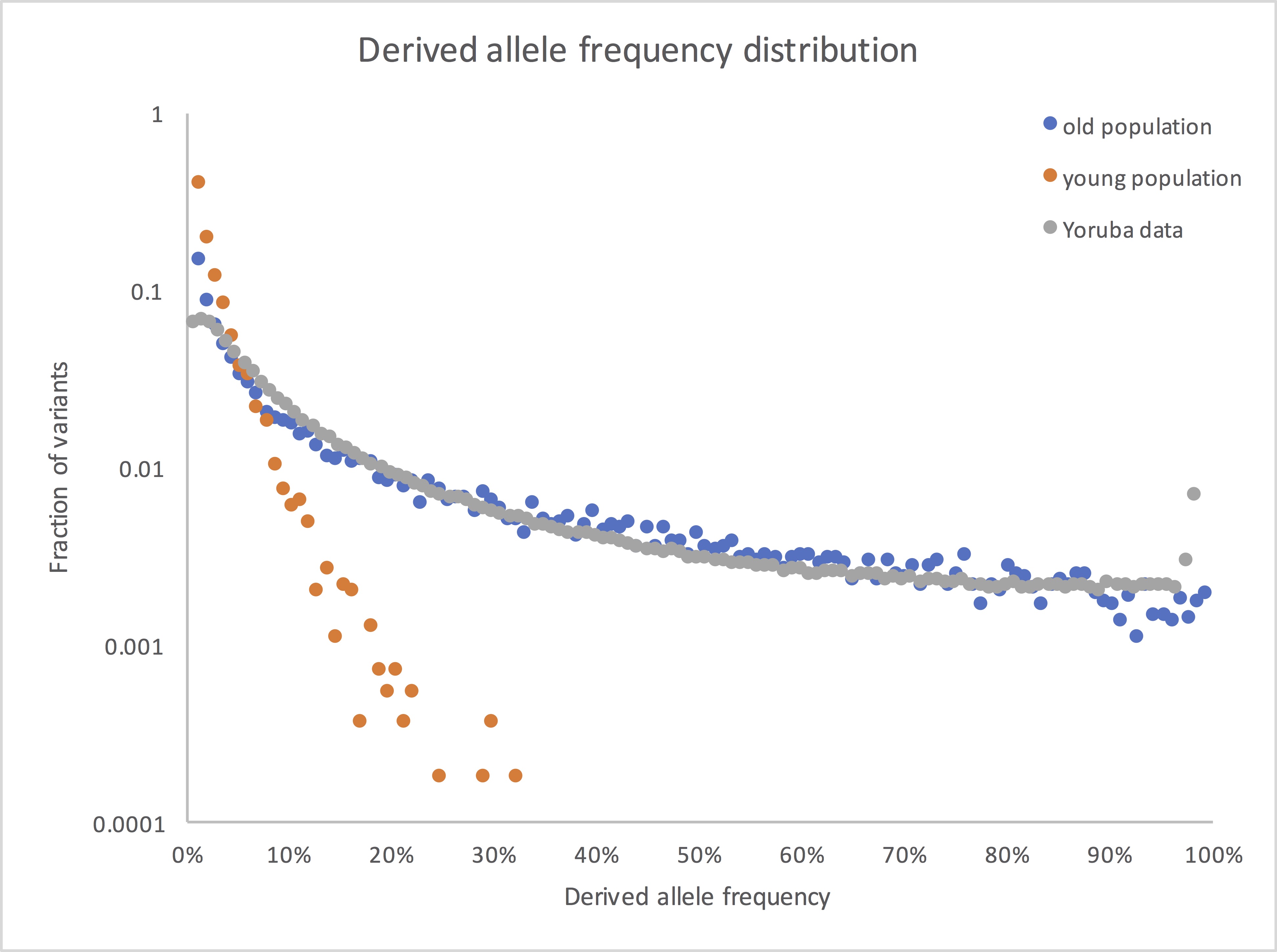
So here’s what the frequency spectrum shows if you compare your young population model with an old population version that’s otherwise the same, along with some West African data from the 1000 Genomes Project:
(I’ve dropped the lowest frequency bin, where 1kG had little power to detect variants. I may also have expanded or contracted the x axis for the real data, since I don’t remember exactly what’s in my own file at this point. But the overall picture is accurate: real human genetic variants look old.)
Thanks this is very helpful. So this is very counterintuitive to me: why are there so many variants with such high allele frequencies? If you look at the young population plot, it’s exactly what I’d expect a random-walk diffusion to look like. High-allele frequencies fall off exponentially. In contrast, the Yoruba data and the old population data barely fall off at all; it looks almost linear. But how does that happen if this is a diffusive process?
For example, when you go from 10% to 20% to to 30% frequency in the young population model, your fraction drops by a factor of 10 and then 100. That makes perfect sense to me, because the variants have to diffuse 2x or 3x as far. In contrast, in the old population model, you diffuse 2x or 3x as far and the variants drop by (maybe?) a factor of 2 or 3. What’s the physical picture behind this? Is the idea that many of these variants have existed at relatively high frequencies (say 30%) for thousands of generations so that we’re not seeing a diffusion from 0%, but from 30%?
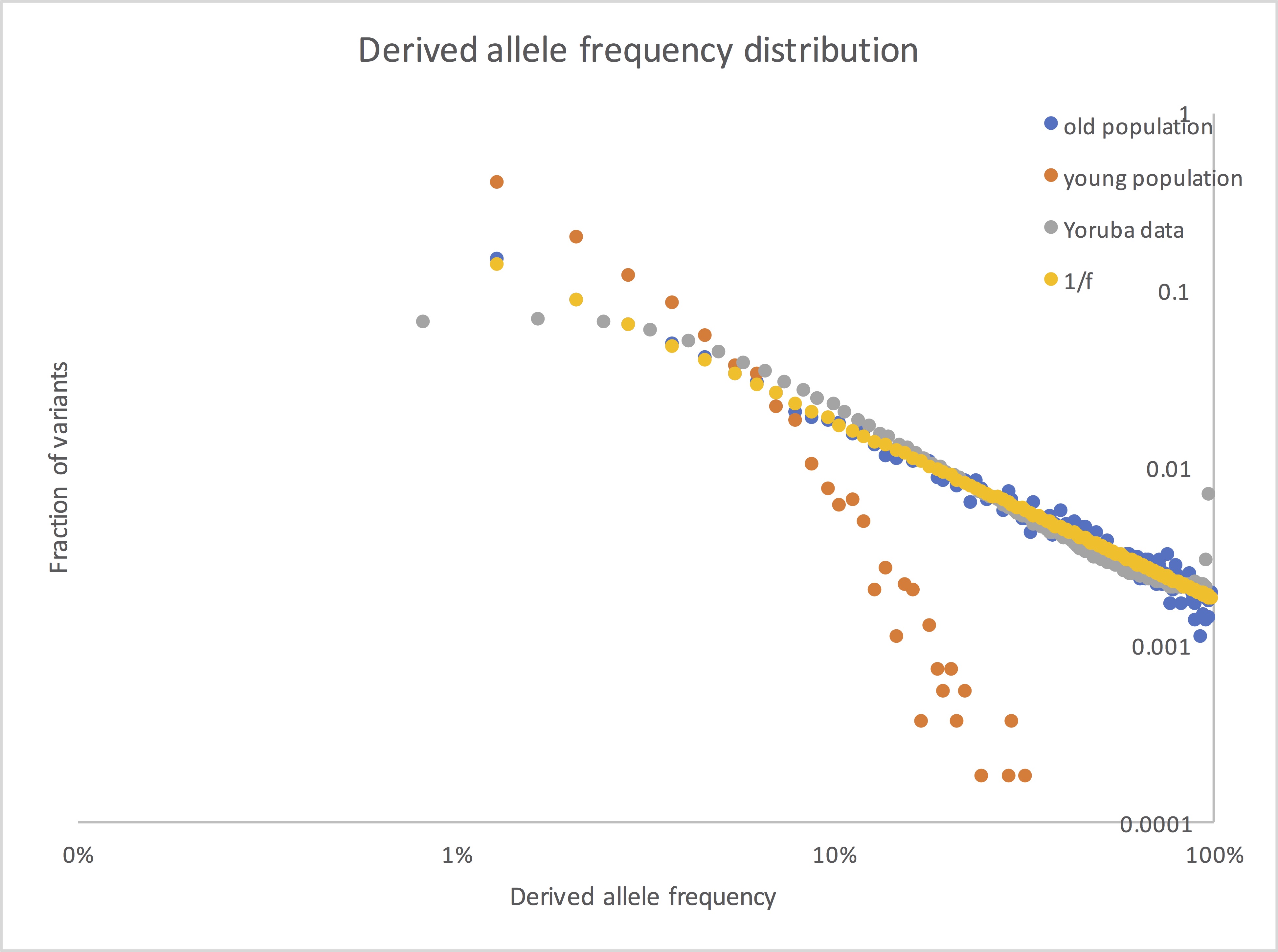
(I just took 1/(center of each bin), which isn’t exactly right, but it’s pretty close for small bins.)
Here it is in a log-log plot, which should make the shape more obvious:
Right. Anything at 40% has to have diffused from 30%. 1/f is indeed what you get from a steady-state diffusion process; Kimura actually derived this (and many other things) from the diffusion equation.
The data ended up in one of the 1000 Genomes papers. (Looking at the dates on my files, it must have been from the pilot phase of the project.) I remember if this was from a final dataset or if some more tinkering happened before release. (If not final, it was close.) If I wanted to do it properly, I’d download the Phase 3 data and calculate from scratch. The data I used here was from SNPs in intergenic regions, since they are less affected by natural selection than those in genes.
Note that I’m only showing the shapes of the distributions, not the overall scale (i.e. not the actual numbers of SNPs); the latter will depend on population size and on the mutation rate, neither known very well. There’s no fitting involved. The simulated distribution is for a constant-sized population (your 10k, in fact) simulated for 20 x (population size); the Yoruba distribution is whatever came out of the sequencing. The Yoruba data is below the simulated for very low frequencies, presumably because of failure to detect low-frequency variants in the low-coverage sequencing we were doing. It’s above it for somewhat higher frequencies, probably reflecting population expansion. It also has a spike at very high frequencies because of alleles that have their ancestral state identified incorrectly; those should actually be at the low end.
1 Like
gbrooks9
(George Brooks, TE (E.volutionary T.heist OR P.rovidentialist))
9
Implicit in the Young Population scenario is that the Young population is still small.
You do know, yes?, that small populations are more easily influenced by mutations? And that large one’s are rather resilient to genetic shift?
This is a well established tendency!
It is only when a population has been so diminished by natural pressures that it becomes more open to novel arrangements of alleles and/or mutations! This is the direct result of an increasingly tightening bottleneck.
Ah, this makes perfect sense. And the total time has to be long enough for the diffusion process to ‘feel’ the other absorbing wall, or you won’t reach steady-state. It’s no wonder my simulations don’t show this, because they treat only one absorbing barrier!
However, I’m not not sure how we get the population size out of this. If 1/f is the signature of a steady-state process, then it should fall out of any size population, as long as we wait long enough, correct? And wouldn’t it follow that the smaller the population, the less time we’d have to wait (I’m guessing that the waiting time is something like 1/N^2, based on solid state physics)?
Also, is the Yoruba data representative of the human genome as a whole?
One more question: I’m now not sure what your ‘old population’ plot represents. In both models, you used t = 20*N on a population of N=10,000, correct? So what distinguishes the models? Did you anneal the ‘old population’ model to reach a steady-state before beginning the simulation?
George, I’m not sure I understand your question. It’s the shape of the tail that was surprising to me, because I didn’t realize that it implied a steady-state diffusion.
gbrooks9
(George Brooks, TE (E.volutionary T.heist OR P.rovidentialist))
12
I believe the shape of these curves correlate proportionally to how large the populations are in relation to the average incidence of new mutations and/or allele ratios vs. how steep the natural selecdtion attrition curve is for the population at a given time.
If the population is small (all things being equal) - - or larger if natural selection attrition is higher than an average baseline - - things happen more quickly than if natural selection attrition is not particularly severe and/or the population is larger.
It’s basic math: the larger the population, and the lower the attrition is for owning the dominant allele configuration, the longer it takes for the population to respond to genetic changes of any kind.
@Swamidass or others here could tell me/us if they think I’m on the right track.
@nashenvi I’m not sure if this is exactly a diffusive process. It is more like a snowball process. The more you grow, the easier it is to grow. The axis obscures this a bit, because it is “fraction of variation” rather than “frequency”.
In the young-pop case, everything should be very low frequency and there are only a few variants. They are all moving at the same rate therefore. In the old-pop model, some of them have grown enough to start snowballing, by fluctuating with higher variance.
Okay maybe snoball isn’t the exact right analogy.
That is why log-log graph shows a line. Do you see that and know what it means? This is a power law or scale-free distribution, a classic feature of many processes, including this. The fact that we see scale-free distributions in DNA is a good indicator that the populations are old.
1 Like
gbrooks9
(George Brooks, TE (E.volutionary T.heist OR P.rovidentialist))
14
The point I was making is that implied in the Young Population scenario is smallness… while an older human population has moved well beyond the relatively tiny dimensions of a founding kin group.
The bigger a population becomes the less affect genetic changes in any given year affects the whole population.
This is what I’m trying to develop an intuition for. But I’m not convinced that there is a ‘snowball effect’ (assuming random mating and no homozygous mutants). Under these assumptions, it’s easy to work out the fact that the probability of increasing or decreasing the frequency of a mutation in a particular generation is independent of allele’s frequency in the population.
[EDIT: Ah, I think I know what you’re saying now. You’re saying that if only 1 individual possesses an allele, then in the next generation, only 2 individuals can possess it. But if 50% of the population possesses an allele, then there is some exponentially small but non-zero, chance that in the next generation, 100% of the population will possess it. So the average expected outcome doesn’t change based on allele frequency, but the variance is much larger. I’m not sure how dramatically it alters the overall dynamics, since these large fluctuations would be extremely rare events (~1/2^O(N)). But I’ll admit that I don’t have a good intuition about this.]
That is why log-log graph shows a line. Do you see that and know what it means? This is a power law or scale-free distribution, a classic feature of many processes, including this. The fact that we see scale-free distributions in DNA is a good indicator that the populations are old.
I know how to read a log-log plot, but I’m still trying to develop an intuition about the meaning in the context of population genetics. For example, why does a power-law distribution demonstrate an ‘old population’? It seems to me that what it demonstrates is that a steady-state condition has been reached. But how long it takes to reach steady state would seem to depend on the population size and the mutation rate, right?
-Neil
1 Like
gbrooks9
(George Brooks, TE (E.volutionary T.heist OR P.rovidentialist))
16
@nashenvi, you write: “It seems to me that what it demonstrates is that a steady-state condition has been reached. But how long it takes to reach steady state would seem to depend on the population size and the mutation rate, right?”
If you understand the words you wrote, then you are in a perfect position to understand why the curve that applies to the genetic diversity of the current human population reflects a starting state that is much older than 6,000 years old - - unless you are going to propose God kept introducing genetic variations in each generation from the time of Adam that had the effect (intentional or not) of presenting human diversity as much Older than 6,000 years in-the-making!
George,
I’m still not understanding your argument. If I understand the significance of the 1/f frequency distribution correctly, it entails that a steady-state has been reached. But reaching a steady-state will depend on the population size. It’s just as possible to reach a steady-state in a population of size N=100 as it is in a population of size N=10,000. If I’m correct in drawing an analogy to solid state physics, the time required to reach steady state should scale something like t = O(N^2) generations (although I could be wrong about this as well; it’s been a while since I did stuff with diffusion).
For example, if we assume an original pair that took 7 generations to reach a population size of N=100, it would then take around t ~ O(N^2) = 10,000 generations to reach a steady-state from which we’d obtain the same 1/f plot (again, assuming I’m correct). So it seems to me that we’d have to make an additional argument that takes into account the absolute number of SNPs, the mutation rate, the population size, etc… to rule out an ancestral pair. Does that make sense?
I think it just depends on the number of generations. This is not steady state. I"m not sure what the cutoff for seeing this is exactly, but is certainly several times longer than 6,000 years for human populations. That much we know, but perhaps 200,000 years might be enough. That is less clear.
Still there are many more than four alleles in common between us and chimps at several places in the genome. That is a very difficult to explain puzzle if we start from a single couple, unless God is specifically introducing chimp DNA into early humans. That is very hard to square with reality.
I
@glipsnort can you give us your graphs without scaling to total population? That might help.
That is the extreme and it is unlikely. I am talking about the more common outcomes. The bigger you are, the bigger steps your random walk takes each generation, and that is what gives rise to the power law distribution in this case. You intuition should be built around that basic logic. It doesn’t have to be “large” fluctuation, but a “larger” fluctuation.
We are not at steady state. I"m not sure what you mean by absorbing barrier.
Also, this is not steady state. There are a steadily growing number of mutations. We are just looking at the relative distribution of SNPs. There is a relationship between the total number of mutations and mutation rate and generation time, but this distribution does not. I think the old population has more generations, that’s it.
Average time to fixation (which is closely related to this) is proportional to N, not N^2. Rate of fixation is independent of N and just depends on mutation rate R.
Your analogy is not really right.
Which is exactly what happens in LD analysis, as described by @DennisVenema in his book so well .
It does not work to “rule out” a pair as much estimate the effective population size. The estimates will be proportional to the geometric mean of the true value, and are therefore biased a bit upwards from the arithmetic mean, but “effective size” so biased down from the “census size”.
An easier to understand and minimum to the population size is from looking of ancient alleles shared by both humans and chimps. In normal circumstances, an individual will carry 2 alleles at a time. If we see more than 4 alleles (e.g. versions of gene) shared between us and chimps, that means we need more than 2 ancestors to carry all that variation. Otherwise, how did human magically get chimp DNA into our genomes that wasn’t in Adam or Eves?
Exon 2 of the DRBJ gene consists of 270 nucleotides that
specify all the (3-chain amino acids involved in peptide
binding. No fewer than 58 distinct human alleles have been
identified that differ in their exon 2 nucleotide sequences.
Fig. 3 is a phylogenetic reconstruction of the 58 alleles.
The time scale has been determined by the “minimumminimum”
method (39, 40), which is based on the comparison
between pairs of species that share the same divergence
node, such as the three pairs orangutan-human, orangutangorilla,
and orangutan-chimpanzee. The minimum distance
observed in such a set of comparisons will correspond to
alleles that diverge at, or close to, the time of the species
divergence. (Alleles that were polymorphic at the time of the
species divergence will show larger distances than the minimum-minimum
value.) A plot of minimum-minimum distances
versus the correspondent divergence times gives an
estimate of rate of evolution.
As can be seen in Fig. 3, all 58 DRBJ alleles have persisted
through the last 500,000 years, but coalesce into 44 ancestral
lineages by 1.7 Myr before present (B.P.), 21 lineages by 6
Myr B.P., and 10 lineages by 13 Myr B.P. It is apparent that
the DRBI polymorphism is ancient, so that numerous alleles have persisted through successive speciation events. In order
to pass 58 alleles through the generations, no fewer than 29 individuals are required at any time. As we shall presently
see, the size of the human populations needs to be much greater than that in order to retain the DRBJ polymorphisms over the last few million years.
To account for the variation this exon alone, there were always more than 29 individuals in the human population.
If you didn’t catch that, there are 58 versions of the DRBJ exon shared by humans, orangutans and chimps. They are identical amongst all three of us. How did they get there if we do not share a common ancestor?
God can do anything, so is certainly possible that God introduced these mutations into Adam and Eve’s children over several generations. It is also possible that he made them mosaics, with different genomes in each of their eggs/sperm. If he did this, he was introducing chimpanzee DNA into our genomes outside the natural order. Either way, the DNA evidence (and the Biblical account) points to a larger population than a single couple.
2 Likes
gbrooks9
(George Brooks, TE (E.volutionary T.heist OR P.rovidentialist))
19
I think you’re conflating common descent with an original ancestral pair. But these are two separate issues. Even on a purely naturalistic account of Darwinian evolution, there’s nothing impossible about a new species originating with a single pair that becomes geographically isolated from a population. I believe that both Dawkins and Coyne talk about this possibility with respect to other species like Galapagos tortoises.
"The bigger you are, the bigger steps your random walk takes each generation, and that is what gives rise to the power law distribution in this case. "
Upon reflection, I think you’re right that diffusion will happen faster at higher allele frequencies, but why think that this is what gives rise to the 1/f distribution?
Also, this is not steady state.
I think “steady state” here refers to the distribution of variant allele frequencies, not the absolute number of variants. That’s why the plots deal only with proportions of variants, not absolute number.
“Average time to fixation (which is closely related to this) is proportional to N”
Can you point me to a derivation of this result? Given the above, I think it seems plausible but it’s very unintuitive to me (it would correspond to diffusion through a material with a viscosity gradient, not something you encounter very often!)
“Otherwise, how did human magically get chimp DNA into our genomes that wasn’t in Adam or Eves?”
Right, but this is again a different argument. The OP was asking about how SNPs relate the original ancestral population.