There are three questions we can ask about what genetic variation would look like if we come from a recent Adam and Eve: what is the total number of genetic variants present today, what is the distribution of their frequencies (e.g., take A/G variants – how often is the A seen in 50% of chromosomes vs. in 5% of chromosomes or 0.1%?), and what are the relative numbers of different kinds of mutation. As Carter notes, the first question turns out to be uninformative: If Adam and Eve were created with different genomes, there could have been any amount of variation already present in the first couple. The mutation model also cannot make a prediction without an independent estimate of the ancestral population size, and so this one is a wash.
When it comes to the third question, about the different kinds of mutations, Carter kind of waves his hands trying to make it go away. He does concede that transitions – which we know occur more often in mutations than transversions – make up the bulk of genetic variants in the human population. This certainly sounds like evidence that the variants are the product of mutation. Actually, the situation is worse for Carter’s model than he acknowledges. There are other ways of classifying mutations than transition vs transversion, and some of them have different mutation rates. In particular, the combination of bases ‘CG’ (that is, a C followed by a G on the chromosome) mutates like crazy, with the C usually mutating into a T. (The reason for this high mutation rate is well understood, by the way.) When we look at genetic variation in humans, we do indeed see a greatly increased rate of C/T variants in the human population when the C is followed by a G – once again what we would expect if all variation originally started out as mutations.
What is disturbing about Carter’s treatment of the question, though, is his logic: “This is not evidence against the creation model, however, as I do not believe the creation model makes any specific prediction about these ratios.” In short, he has the mutational model, which predicts very specific things about genetic variation, and the creation model, which predicts nothing. When we see the predictions come true, we are not allowed to conclude anything, though, because one of the models didn’t make a prediction. To this I can only say, “Huh?”
(On this last point, a parable: There was a town in which the police were trying to bring a criminal gang to justice. One evening, a man appeared at the police station and told detectives that he had inside information on the gang, and that he could supply it to the police in exchange for cash. “Prove it,” the detectives responded. So the man told them, “That murder last week – I know who did it. I don’t know his name, but he’s a left-handed man in his late forties, balding and with a beard and he’s got a tattoo of a star on his left bicep. Oh, and he speak Lithuanian.” Well, the next day the police happened to catch the murderer, and he did indeed turn out to be a star-tattooed left-handed Lithuanian etc. When the informant returned, though, the police told him this: “We have two theories. Theory 1 says you don’t have inside information, while theory 2 says you do. If theory 2 is correct, then your information about the murderer will be accurate. If theory 1 is correct, then we wouldn’t know anything about the murderer despite what you told us. Since theory 1 doesn’t make any predictions about the murderer, we have no way of judging whether you knew who he was or not.” And so the reign of terror continued.)
It is on the second question, though – the frequency distribution of genetic variants – that Carter really screws the pooch(*). There’s nothing obviously wrong with his simulation of what to expect from accumulated mutation: we really should find lots more rare variants than common ones. In an ideal, constant-sized population, in fact, the number we find would drop off as 1/f, where f is the frequency of the new, mutated variant (in technical language, of the “derived allele”). That is, if we find 1 variant occurs in 40% of the population, we would find 2 that occur in 20% of the population, 4 that occur in 10% of the population, 8 in 5% and so on, down to very low frequency variants, of which there will be very many.
Carter’s problem lies not in the simulation but in the data he is contrasting with it (see his Figure 2). What he is using is HapMap data for a European population; he finds that the distribution is nearly flat. There are two problems here. First, while humans as a whole haven’t been through a substantial population bottleneck in our recent genetic history, European populations have been through one or more, including a pretty tight one when humans left Africa before ending up in Europe. Bottlenecks have the effect of flattening out allele frequency distributions. So no fair comparing this to the simulattion.
More importantly, what he is plotting is not the frequency distribution of all variants in the European population. Instead, it is the frequencies of variants that the HapMap project chose to study. They chose the variants by identifying them in a small ascertainment sample (which greatly favors higher frequency variants) and selected them for being present in multiple populations (same effect). This guarantees major distortions to the frequency distribution. (This also means that the HapMap data were very hard to use for inferring population history or other population genetics purposes. I was part of the HapMap project when these decisions were being made, and the population geneticists were not happy.)
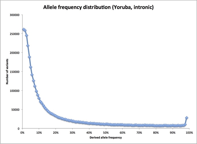
What he should be doing is looking at all variants found in a sample of an African population, which requires determining the full sequence of each individual. Fortunately, this has been done as part of the 1000 Genomes Project. I happen to have a spreadsheet with data from early in the project on my laptop. (Better data are probably available now, but this set is fine for this purpose.) Here’s the actual frequency distribution for the 1000 Genomes sample from the Yoruba, a West African population:
As you can see, the real distribution does indeed fall off quickly at higher frequencies – as we would expect if the human population had been large for a long time. (Note: the little sag at the very left of the plot is because the 1000 Genomes sequencing was not very good at finding really rare variants. The odd blip at the far right are variants where I have picked the wrong variant as the derived allele: they belong all the way on the left end instead. Their loss from that end also contributes to the flattening out there.)
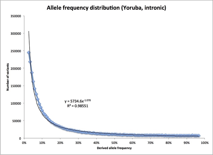
In fact, we can see how similar the actual distribution is to that perfect, 1/f distribution for a constant-sized population I mentioned before. Dropping the first bin and the last two bins (for the reasons noted above), and fitting a simple power curve, I find this:
Instead of falling as 1/f, that is, f to the power -1, it falls slightly faster, as f to the power -1.078. Not bad at all, especially since there is no reason to thing the ancestral human population was actually constant in size.
In short, had Carter examined a suitable data set, he would have found that his model was completely untenable.
(*) Probably not suitable language for a 5 yo. Tough titty.

