This is important conversation for a lot of people. It also has been useful.
Can you clarify what you are getting at here?
What exactly are the exotic effects from the Lenski experiment that (1) apply to large mammals like humans, and (2) are capable of dramatically affecting TMRCA estimates?
The key formula we are relying upon to compute times is D = R * T, or the number of differences equals the product of mutation rate with time. This formula is expected to hold best in non-coding regions of the genome, when there is not balancing selection.
Look at figure 2 from the Lenski paper, which shows how mutation rate varies in each experiment. Look at panel B.
Here we can see there are two groups. One group (red and orange) are mutators, that at some point start rapidly mutating much more than the normal rate. One group (blue - purple) are non-mutators which are just mutating a a more normal rate. The key point is that there is a wild difference between these two groups.
However, this wild of variation in mutation rates is not relevant to mammalian populations. There is much much more constraints on mammalian germline mutation rates, and we do not see such wild swings between populations. So this is an example of an effect in the Lenski experiment that we do not need to account for when studying human DNA. Adding to that pattern, we know that much more of the human genome is non-coding than in bacteria, so it will be more clock like too.
Yes, we do expect some variation, but it’s hard to imagine that variation being more than just 10 to 20% when averaged over 10s of thousands of years.
Also, we are using a median estimate TMR4A, so even if some regions of the genome behave weird (e.g. because of balancing selection) they have no effect on the results. So can you clarify what specific effects you think will substantially reduce our confidence in the TMR4A estimate I gave? As I understand it, the confidence intervals I’ve put forward are gestimates, but they do take into account everything relevant from the Lenski experiment. Let me know what I am missing.
I’m not sure what is unclear. I’ve already explained that they are not estimating Ne, but have a weak prior on the trees computed using Ne. They do not estimate Ne in the past, nor do they assume specific value.
Let’s not be too dismissive.
I think this analysis seems to be pretty strong evidence against a single couple before, say, 300 kya. It does not tell us if a bottleneck happened after 500 kya, but it seems to indicated one did not happen after. It is just a simple formula that is relevant here: D = R * T. We can directly measure D and R (number of differences and mutation rate). So no real leaps are being made.
You’d have to specify more carefully what effects need to be better modeled, and give good reason to believe this would substantially alter the results. I’m all for questioning the data, but I cannot imagine plausible model with a couple at (say) 100 kya. I trust you agree with me on that, right?
If you are referring to the value of a recent genealogical Adam to the theological debate, I agree with you. That option seems like it will have a bigger impact on the conversation. That model has a great deal of consilience with the Biblical record and is 100% consistent with the genetic data.
However this question about a single couple bottleneck is important too, because it seems we are coming to a consensus that a single couple bottleneck before about 300 kya (taking into account the uncertainties in a TMR4A of 500 kya) is very unlikely. @RichardBuggs is pressure testing it now, but I trust he will eventually acknowledge this point. The way we constructed that estimate (as a median across the genome), it will not be susceptible to most of the concerns that have been raised. The evidence here is pretty strong (though I do not make any “heliocentric” statements). Nonetheless, this opens up the possibility of an ancient bottleneck (say at 600 kya or 2 mya), for those who feel it’s necessary.
Rather than prosecuting that TMR4A value I computed ad nasueum, I think a better idea would be to turn to trans-species variation. Of course, there will be better estimates of TMR4A in the future, but the conversation might be better served by looking at another class of evidence.
Woah, I was taking for granted that of course we have evidence of various pre-humans! Perhaps I shouldn’t have assumed though. Do you want to talk about any in particular?
The scenario of a bottleneck in one species, followed by interbreeding with a related species would not be nearly as obvious genetically because the genetic diversity would be lowered by the bottleneck and higher due to inbreeding. We would have to be able to pick out which genetic material came from the interbreeding somehow. Not impossible, but complicated.
Luckily usually when we speak of a bottleneck we simply mean a bottleneck of all ancestors of a given organism, whether they are one species or not.
I’m unfamiliar with this modeling, do you have a link?
Doesn’t this need a qualifier, according to this particular line of evidence? I know there are other topics than TMR4A which have yet to be discussed in detail.
@gbrooks9,
No, a single couple for multiple generations would be losing genetic diversity fast with each generation, very unhealthily. I think we’re assuming Adam and Eve could’ve had different genes from each other.
@Swamidass,
Thanks for the correction! I am very sorry to hear about your father. I appreciate the time you are taking for this thread!
A search of my folder on this blog provided the following:
Let me know if this is sufficient.
The difficulty I am experiencing when I try to follow the discussion is to imagine a bottleneck for the model of one species, when it may be that a number of (pre)humans may need to be modelled with individual bottlenecks - I assume the various species would not mingle - however I hasten to add that I will not pretend to comprehend the basis of this modelling, as it seems to be vastly different to computer modelling/simulations I have carried out.
Perhaps the various (pre)humans did mingle, but again, should the model take some sort of physical data that would show if such existed at the same time, or various times; or are we assuming the human species we presently examine wrt genetic diversity just emerged from a mixture in the distant past.
I again emphasise that my interest is in linking the strange modelling of genetic diversity with the point of this discussion of what catholic Christianity terms truly humans, and of course Adam and Eve. My impression is of a complicate past, a lot of which cannot be verified within these models (but obviously of interest to workers on population genetics).
To be clear, this is about our common ancestor, but not our sole common ancestor: it would be Adam and Eve within a population of other humans that their children married into.
I don’t quite understand. We would need DNA with which to do this modeling, yes? And the only living descendants of any post-chimpanzee-split hominins are us, modern humans. We have also managed to retrieve a little Neanderthal/Denisovan DNA, but we can’t genetically model lines we don’t have DNA from.
Like I said above, it is complicated but possible to pick out DNA which seems to have come from interbreeding events, and we do find such evidence of interbreeding with Neanderthals and other older populations which we have not yet matched with fossil evidence. These findings are still pretty recent.
I’m still not sure I’m getting at what you’re asking, but I’ll agree with you that it’s complicated!
Sorry to reach all the way back to this old post, but it seems to me that the following paper is pertinent, since they present a new method of calculating past population sizes.
The abstract: Inferring and understanding changes in effective population size over time is a major challenge for population genetics. Here we investigate some theoretical properties of random-mating populations with varying size over time. In particular, we present an exact solution to compute the population size as a function of time, Ne(t), based on distributions of coalescent times of samples of any size. This result reduces the problem of population size inference to a problem of estimating coalescent time distributions. To illustrate the analytic results, we design a heuristic method using a tree-inference algorithm and investigate simulated and empirical population-genetic data. We investigate the effects of a range of conditions associated with empirical data, for instance number of loci, sample size, mutation rate, and cryptic recombination. We show that our approach performs well with genomic data (≥ 10,000 loci) and that increasing the sample size from 2 to 10 greatly improves the inference of Ne(t) whereas further increase in sample size results in modest improvements, even under a scenario of exponential growth. We also investigate the impact of recombination and characterize the potential biases in inference of Ne(t). The approach can handle large sample sizes and the computations are fast. We apply our method to human genomes from four populations and reconstruct population size profiles that are coherent with previous finds, including the Out-of-Africa bottleneck. Additionally, we uncover a potential difference in population size between African and non-African populations as early as 400 KYA. In summary, we provide an analytic relationship between distributions of coalescent times and Ne(t), which can be incorporated into powerful approaches for inferring past population sizes from population-genomic data.
They call their method POPSICLE and describe it as such: There are two important steps for most of these types of approaches: the inference of the underlying gene genealogies and the inference of population size as a function of time from the inferred genealogies. In this article we introduce the Population Size Coalescent-times-based Estimator (Popsicle), an analytic method for solving the second part of the problem. We derive the relationship between the population size as a function of time, Ne(t), and the coalescent time distributions by inverting the relationship of the coalescent time distributions and population size that was derived by Polanski et al. (2003), where they expressed the distribution of coalescent times as linear combinations of a family of functions that we describe below. The theoretical correspondence between the distributions of coalescent times and the population size over time implies a reduction of the full inference problem of population size from sequence data to an inference problem of inferring gene genealogies from sequence data. This result represents a theoretical advancement that can dramatically simplify the computation of Ne(t) for many existing and future approaches to infer past population sizes from empirical population-genetic data.
Data and code availability are given in the paper:
Simulated data can be regenerated using the commands given in File S1. Data from the 1000 Genomes Project are available on the ftp server ftp://ftp.1000genomes.ebi.ac.uk/vol1/ftp/. Code for the computations is available at: jakobssonlab.iob.uu.se/popsicle/.
Don’t know if any of this is helpful, but it seemed pertinent, at least.
Thanks for your thoughtful responses. I will try to repond to you on the three issues we are now discussing about Ramussen et al 2014: (1) estimation of Ne (2) estimation of recombination rate (3) “exotic effects”. This may be quite a long post, or may have to end up broken in to a series of three!
(1) Estimation of Ne
Here, I am responding to your post #457Adam, Eve and Population Genetics: A Reply to Dr. Richard Buggs (Part 1) - #457 by Swamidass Your post discusses two issues, the prior on time (T) and the prior on Ne. Here I am only concerned with Ne. I still think that the footnote in the paper under Table 1 shows that even though ARGweaver can allow for changes in Ne, they did not use this ability in their analyses of the human dataset. They say “Model allows for a separate Ni for each time interval I but all analyses in this paper assume a constant N across time intervals.” I think that you have examined the code, and are rightly saying that the code can allow for changes in Ne, but you also need to take this footnote into account that says that Ne was kept constant in their analyses. I think that the effect of this will be to push back the TMR4A. If they had assumed that the human population had increased from a single couple to 7 billion individuals, I think the median TMR4A would be lower.
My original point here was that all our methods (that I know of) that calculate Ne from genetic diversity will give a high value of Ne over the time period of a short, sharp bottleneck. However, this does not mean that if there were such a bottleneck it would not have profound population genetic effects even if it were undetected by our methods. It would cause sharp increase in the number of coalescence. I think (though I am not completely sure) that @DennisVenema may be correct in his Part 2 blog in response to me that 25% of polymorphic genes will have coalescence events at a bottleneck of two. However, I think that these will be hard to detect, as the inaccuracy of our estimates of TMRCAs will mean that the coalescence events will appear to us with our estimates to be smeared out over a longer period of time and we will detect a small drop in Ne, rather than a bottleneck (BTW, this is one reason why PSMC struggles to detect bottlenecks).
So I think what I am saying is that even if in the real history of a population there is a short sharp bottleneck that causes a burst of coalescence, we will struggle to pick that up, and thus will thus miss the bottlenecks and the effects we might expect it to have on rates of coalescence. This argument is assuming a method that allows estimation of coalescence times and Ne, with feedback between the two, but this is not what ARGweaver does, so this is a slightly academic conversation in this context. As you say, ABC methods are better at modelling Ne and TMRCA at the same time, but my experience of this is that the two variables are so dependent on each other that it is hard to know for sure what is the effect of time and what is the effect of population size – but this is a separate discussion that is not really relevant to the Ramussen et al paper, which is not modelling Ne.
The purpose of argweaver is not to estimate Ne, so they do not estimate it. They instead are estimating phylogenetic trees. The times on trees is determined not by population modeling but by the formula:
D = R * T
The only way Ne affects things is by putting a weak prior on T, but this prior is lower than that which is measured. So we know that the prior only reduces the TMR4A estimate.
@RichardBuggs I have taken that into account and said exactly the same. Moreover, I have shown that their choice of Ne reduces the estimate of TMR4A, not increases it. One what basis are you disagreeing here?
Its the exact opposite. If they had chosen a larger Ne, the estimated TMR4A would be higher, by a small amount. I’m not sure how you are forming your intuitions here. As I’ve explained, I’ve looked at the code carefully. What I first wrote about this still applies…
Which once again gets to a key point…
That is just as I’ve explained, but does not reduce confidence, because ArgWeaver is not attempting to estimate Ne. It is merely measuring the trees (i.e. the D in the formula above), while taking recombination into account.
@RichardBuggs I’d quickly acknowledge if I’d made a mistake here or if you have a point. Honestly, however, I am not seeing your point. I think the 500 kya (with about 20% CI) is a pretty solid lower bound on a single couple origin. I hope you’ll agree so we can move on to more interesting data.
That is accurate. Which is why I need to do the simulations to test this. I think this will push a plausible bottleneck back to about 800 kya, but I’m not sure.
Yeah I agree with this.
On a theoretical note, I think there will be a relationship between the distribution of TMR4A, TMR3A, and TMR2A and the time range under which a bottleneck is detectable. The fewer lineages at a particular point in time (which reduce the farther back we go), the less of an increase in the coalescent rate.
You are right though that a sharp bottleneck will not be observed as sharply by PSMC, or really any coalescence based method, including ABC. I agree, it is hard to tell what is the effect of time (length of bottleneck) and population size. From a theoretical point of view, both have the exact same impact on coalescence rate, so it appears they are indistinguishable by looking at coalescence rate alone.
Closing out on TMR4A.
The reason why we measured TMR4A is because it provides an easy to understand lower bound, and is easier to robustly measure with fewer assumptions than coalescent rate (which is a second order or third order statistic). If there is a single couple bottleneck, we should no more than 4 lineages when it occurs.
One again, I do hope you can endorse that finding. In the end, it proves your critique of Venema is essentially correct.
Of course, we can imagine better ways of measuring TMR4A. When I get around to it, I might make some improvements myself. However, what’s been put forward is a solid starting point that is not going to see wild revisions downwards without large changes to mutation rate.
(2) Recombination rates and TMRCA estimated in Ramussen et al (2014)
Thank you @Swamidass for the information that the ratio of mutation rate to recombination rate (mu/rho) used in the ARGweaver analyses of human population data is around 1.13. My reading of the paper is that this means that (as Joshua has also said) they will miss some recombination events. I agree with Joshua that:
However, I think that the lack of detection of other recombination events will have an effect of the TMRCA, causing it to be overestimated.
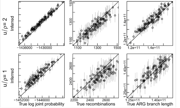
Here is part of Figure S4 from the paper:
Note that it is the lower set of charts that is for the value of mu/rho that is closest to 1.13. This shows (middle row) that the number of recombinations is systematically underestimated by ARGweaver with this low mu/rho value, and the error in estimating branch lengths is higher than would be the case if mu/rho were higher.
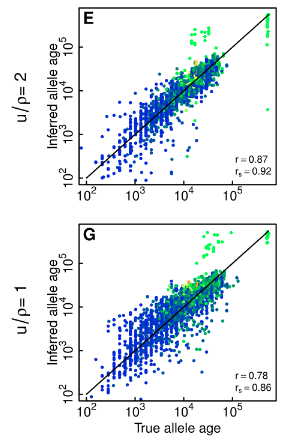
Here is part of Figure S7
This shows that the error in estimating allele age is greater at mu/rho = 1 than at mu/rho =2 . Whether or not there is a degree of systematic overestimation of allele age at mu/rho=1 is hard to tell from eyeballing the chart as we can’t see the density of the clusters very well. There is a cluster of alleles with high derived allele frequency (coloured green) that have a true age of under 10^5 but are estimated to have an age of over 10^5 and this effect is greater at mu/rho = 1 than at mu/rho = 2.
It is also worth noting from Figure S8 that at mu/rho = 1 only about 60% of tree topologies are correct in ARGweaver. My guess is that incorrect trees are likely to be less parsimonious than correct trees, and so would elevate the TMRCA.
The main point I was making from the Lenski experiment is this:
I agree with your point that a “mutator” phenotype as extreme as those seen in some of the Lenski populations is unlikely/impossible a human population, and that you have done your best to account for the effects of balancing selection.
However, we do know that mutation rates can vary to some extent between human populations. As Kelley Harris wrote recently in Science http://science.sciencemag.org/content/358/6368/1265.2.full
“it is very clear that some mutagenic force became overactive in the European population during the past 20,000 years or so since Europeans and East Asians started differentiating into separate populations.
This contradicts the popular “molecular clock” model (13), which posits that mutation rates evolve very slowly over perhaps tens of millions of years. Rather, it suggests that DNA replication fidelity is a lot like other biological traits, sometimes evolving by leaps and bounds for reasons that usually elude us.”
Notice that there is still a strong correlation between the estimated and true TMRCA. Also, most of the genome has a u/p > 2, so most of the time the correlation will be stronger than the u/p=1 plot indicates.
I agree that these are sources of error, but I do not think they take the uncertainty much beyond +/- 20%.
What do you think the error rate is? Would you say 20% too, or 30%? Or what exactly? It would be helpful if you would attempt to quantify your degree of uncertainty about these numbers. Perhaps we are not even disagreeing at this point. To what extend do you think these factors increase the spread of our TMR4A estimate?
can the modelling be calibrated in some manner so that one may obtain a method for assessing errors?
I am interested in why accounting for genetic diversity by modelling some type of past and non-verifiable event(s) is treated with such certainty re past events by some proponents on this site.
amen to that brother, and I would add, uncertain as a way of providing a history of the human population over lengthy periods.
Thanks for the reference @Swamidass. This adds to my impression of a very complicated simulation, and I note this goes back a few thousand years - I have paste two portions that may be helpful to this discussion.
gbrooks9
(George Brooks, TE (E.volutionary T.heist OR P.rovidentialist))
483
I have to wonder about this pair of sentences:
“… [it] does not mean that if there were such a bottleneck it would not have profound population genetic effects…” < [ Meaning, it could have profound genetic effects ]
“… even if it were undetected by our methods.”
How profound could the effects be if we couldn’t detect them?
What would be an example of such a profound effect?
I thought this post required a more detailed follow up…
This is a great hypothesis but it is not borne out in the data marshaled. It confirms, instead, my point that the effect is only small on TMRCA. At the core of this is misunderstanding of the statistics at play.
Case in point is S4:
Look at the last column where it shows the true ARG branch length. We see that the variance of the estimate increases but there is no systematic error that is shifting estimates upwards from the true value. This is a critical point. Remember we are taking the median of the TMR4A, which only depends on where the distribution is centered, not its spread. That is why we chose median, not mean. This graph is very strong evidence that the recombination inference errors are NOT increasing the TMR4A, just as I hypothesized.
In fact, even when recombinations are underidentified (bottom row, middle column), ARG length is still measured about the same, but with higher variance (bottom row, right column). We chose an estimator that does not depend on variance, however, so this has zero impact on TMR4A.
We see the exact same pattern in S7. Even though you write…
The correlation between the true and estimated TMRCA drops a little, from 0.87 to 0.78, but if there is systematic error, it is very low. We cannot tell precisely this graph, but we can from the prior graph. The median of each distribution is going to be very close to each other. Taken with the prior figure, this is evidence that the under inference of recombination is not a major source of error. In fact, these data points show that recombination inference mistakes do not change the average/median TMRCA estimates. Also, TMRCA has much higher variance than TMR4A, and TMR4A will be even less susceptible to these types of errors.
In the end, these figures validate pretty clearly my alternate hypothesis, which I formed based on knowledge of how this algorithm works.
Remember, I am a computational biologists, and I build models for biological systems like this in my “day job,” so I am working from a substantial foundation of firsthand experience in how these algorithms work. This is not an appeal to authority (trust or distrust me as you like), but an explanation of why I had some confidence in this in the first place. What we see is what I guessed. There is increased variance in the estimate, but no clearly evidence that the TMRCA is increased more than it is decreased.
This hypothesis seems false. We can see from figure S4 and S7 that about 50% are less parsimonious than the correct tree (higher TMRCA) and about 50% are more parsimonious (lower TMRCA). Remember, we do not expect the trees to be precisely correct. There are just estimates, and we hope (with good reason) that the errors one way are largely cancelled by the errors the other way when we aggregate lots of estimates.
Finally, we are aggregating a lot of estimates together to compute the TMR4A across the whole genome. This is important, because by aggregating across 12.5 million trees, we reduce the error. While our estimate in a specific part of the genome might have high error, that error cancels out when we measure across the 12.5 million trees. This is a critical point.
The statistics here substantially increases our confidence in these numbers.
Just about any source of error we can identify will push some of the TMRCA estimates up and some of them down. However, because we are looking at the median of all these estimates, this increase in variance does not affect the accuracy much. A great example of this is mutation rates.
Yes, there is variation in mutation rate. We can measure it in different populations, and we can even detect some differences in the past. These variations, however, in humans are all relatively small. These variations, also, are not always to higher mutation rates, but also to lower mutation rates. So yes, it is likely that mutation rates were slightly higher in particular populations or points in the past (let’s say within 2-fold per year), but it is also likely they were slightly lower at times too. For the most part, this just averages out over long periods when looking at the whole human population. That is not 100% true, but the law of averages is why variation in mutation rate is not going to dramatically increase our confidence interval on TMR4A by much.
Let’s remember why we are here:
I think it’s fair to say at this point that I did rigorously test the bottleneck hypothesis. Right?
Perhaps there will be improved follow on analysis that will refine my estimates, and I encourage that. However, TMR4A is a feature of the data. It is the length (in units of time, computed by mutational length / mutation rate) of the most parsimonious trees of genome wide human variation. This is not an artifact of a population genetics modeling effort. Rather, it is a way of computing the time required to produce the amount of variation we see in human genetics.
Also, this analysis is very generous to to the bottleneck hypothesis. Though I’m not certain yet (and plan to do the studies to find out), bottlenecks going back as far as 800 kya might be inconsistent with the data we see. There are some large unresolved questions about how a bottleneck effects coalescence rate signatures before the median TMR4A, and if they are detectable.
I hope there can be some agreements on these points, as a conclusion to this portion of the conversation would be valuable. It would be great to move on to more interesting data.
I should also add that the referenced supplementary figures (S4 and S7) appear to be using only 20 sequences. Accuracy improves dramatically as more sequences are added. For the data we used, there were 108 sequences, so we expect better accuracy than the figures shown.
Also, S6 is an important figure, that shows the inferred vs true recombination rates for simulation using the known distribution of recombination rates across a stretch of the genome.
For most of the genome, recombination rate is low (corresponding to high u/p), but only is jumps up at recombination hotspots (the places where u/p is low).
The model picks up some of the recombinations, but not all of them. Most of the recombination inference errors are there, in the recombination hotspots, which are confined to a very small proportion of the genome.
At recombination hotspots, the trees will span shorter amounts of the genome than the rest of the genome. Trees with low bp span are signature for high recombination rate.
That means that most of the genome has a high u/p and is being estimated accurately, but there is only difficulty at recombination hotspots where u/p is low.
By weighting trees by the number of base pairs they cover, we can dramatically reduce any error that might be introduced by recombination inferences. That’s because recombination hotspots are were the vast majority of the errors are, and these hotpots are just a few percent of the genome.
And that is exactly what I did. Rather than reducing the TMR4A estimate, downweighting the error prone recombination hotspots (by weighting by bp span of trees) increases the TMR4A estimate.
I’m going back over all this to point out I was already thinking about the effect of recombination and correcting for it in a plausible way. There are always sources of error in any measurement. This is no exception. The fact there is error however, does not mean the error is large. Clearly, we are only computing an estimate, but this is a good estimate of TMR4A.
Of note, correcting for recombination errors by downweighting recombination hotspots increases the TMR4A estimate. It does not decrease it. Thats because for trees spanning only short segments of the genome, they will be more influenced by the prior. That’s because in short segments of the genome, there is not enough data/evidence to overwhelm the prior, so it takes over. On longer genome segments, the data is strong enough to disagree with the prior. As we have seen, the prior pull the TMR4A estimates downwards on real data. So in the end, reducing the effect of recombination hotspots just increases the TMR4A estimate. This is appropriate, because we want the TMR4A least dependent on the prior.
This may seem surprising, and in conflict with the the S4 and S7 data. It is not. In the S4 and S7 experiments, the prior matched the simulation, and did not pull the results up or down. In the real data, the prior pull the TMR4A estimates down, and pulls them down most in recombination hotspots because their bp spans are smallest. So this counterintuitive effect makes sense as an interaction with the prior and recombination hotspots. This error is important to understand, because unlike most types of errors:
it is biased in one direction (towards artificially lowering TMR4A)
its impact is large (about 70 kya, or about 15% relative effect)
Note, also, that I identified this source of error and corrected for it several weeks ago. Even in my first estimate, I disclosed it was going to be an issue.
Before I looked at the prior, however, I guessed wrong on the direction of the effect. I cannot identify any other sources of error likely to have this large an effect. Also, this adjustment was within my +/-20 confidence interval, which shows even my original estimate was not overstated.
Moreover, I have at this point corrected for it. A better correction might take this further, by just excluding the trees with small bp lengths, thereby excluding all regions where recombination rate is high. This refinement, will certainly increase the TMR4A estimate. I’m more inclined to improve this estimate with a different program first. That would likely have more value in the long run.
Hi Joshua,
Thank you for your patience with me regarding Ne and ARGweaver. I think I have misunderstood something, and I am just having more of a think about this. As I go back over your posts, I am struck by how many times you have made the same point to me, without me really taking it on board:
Sorry I have not taken this on board sooner! Can I try to paraphrase this. What you seem to be saying is that they are simply taking a molecular clock approach to estimating TMRCA. Time is the number of differences divided by the mutation rate. They are building phylogenetic trees and dating them.
The reason why I have been so preoccupied with Ne is because I thought this was a coalescent analysis, where time to coalescence is proportional to effective population size. The bigger the population size, the longer it takes to get back to a MRCA, even in the absence of mutation. The reason why I was thinking that a bottleneck followed by exponential population growth to 7 billion individuals would reduce TMRCA in such an analysis is encapsulated in this figure from Barton et al’s textbook “Evolution” published by CSHL (note especially part C)
If ARGweaver is not doing coalescent analysis in this sense, then I can see that Ramussen et al are simply taking a molecular clock approach, as you seem to be saying.
I am not sure that you are saying that exactly though, as you also seem to be saying that the Ne value they choose is placing a prior on the TMRCA:
This sounds to me like a coalescent analysis, not a simple phylogeny and molecular clock.
I’m sorry, but I seem to be misunderstanding something here.This is why you have had to repeat yourself so much, and I am sorry it is taking me so long the understand what is going on here.
2 Likes
gbrooks9
(George Brooks, TE (E.volutionary T.heist OR P.rovidentialist))
487
Inferring Past Effective Population Size from Distributions of Coalescent Times
by Lucie Gattepaille, Torsten Günther,and Mattias Jakobsson
Abstract
Inferring and understanding changes in effective population size over time is a major challenge for population genetics. Here we investigate some theoretical properties of random-mating populations with varying size over time.
In particular, we present an exact solution to compute the population size as a function of time, Ne(t), based on distributions of coalescent times of samples of any size. This result reduces the problem of population size inference to a problem of estimating coalescent time distributions.
To illustrate the analytic results, we design a heuristic method using a tree-inference algorithm and investigate simulated and empirical population-genetic data. We investigate the effects of a range of conditions associated with empirical data, for instance number of loci, sample size, mutation rate, and cryptic recombination.
We show that our approach performs well with genomic data (≥ 10,000 loci) and that increasing the sample size from 2 to 10 greatly improves the inference of Ne(t) whereas further increase in sample size results in modest improvements, even under a scenario of exponential growth. We also investigate the impact of recombination and characterize the potential biases in inference of Ne(t). The approach can handle large sample sizes and the computations are fast. We apply our method to human genomes from four populations and reconstruct population size profiles that are coherent with previous finds, including the Out-of-Africa bottleneck. Additionally, we uncover a potential difference in population size between African and non-African populations as early as 400 KYA.
In summary, we provide an analytic relationship between distributions of coalescent times and Ne(t), which can be incorporated into powerful approaches for inferring past population sizes from population-genomic data.
@RichardBuggs thanks for your last post. I think you honed in on the point of confusion. Thanks for elucidating it.
You are right, that is the key point. I’m glad we are getting chance to explain it.
That is exactly right. That is what they are doing, with a few bells and whistles. Essentially, this is exactly what MrBayes does (http://mrbayes.sourceforge.net/), except that unlike MrBayes, ArgWeaver can handle recombination. Technically, it is constructing ARGs (ancestral recombination graphs), not phylogenetic trees. ARGs (of the sort argweaver computes) can be represented as sequential trees along the genome. That’s convenient representation that is easier for most of us to wrap our heads around, but the actual entity it is constructing is that ARG.
Except, as you are coming to see, this is not a coalescence simulation at all.
To clarify for observers, there are three types of activities/programs relevant here.
Phylogenetic tree inference. Starting DNA sequences → find the best fitting phylogenetic tree (or ARGs when using recombination) → assign mutations to legs of tree (or ARG) → use #mutations to determine length of legs. (see for example MrBayes)
Coalescence simulation. Starting from a known population history → simulated phylogenetic trees (or ARGs when using recombination) → simulated DNA sequences. (see for example ms, msms, and msprime)
Demographic history inference. Many methods, but one common way is compute #1. Starting from DNA sequences → Infer phylogenetic trees / args (task #1) → compute the coalescent rate at time windows in the past → Ne is the reciprocal of the coalescent rate. (see for example psmc and msmc).
It seems that there was some confusion about what ArgWeaver was doing. Some people thought it was doing #2 or #3, but it is actually just doing #1. The confusion arose because it used a fixed Ne as parameter, which seemed only to make sense if it was doing #2, and might make its results suspect if it was doing #3. However, ArgWeaver was never designed to do #2 or #3. Instead, it is doing #1.
So what is the Ne for? One of the features of ArgWeaver is that it uses a prior, which is good statistical practice. They were using Ne to tune the shape of the prior, but ultimately this does not have a large effect on the trees. It’s only important, in the end, when there is low amounts of data. As I’ve explained several times too, the prior they used pushed the TMR4A downwards from what the data showed too.
How This All Gets Confusing…
In defense of the confused, one of the confusing realities of population genetics is that the same quantities can be expressed in several different units. Often they are all used interchangeably without clear explanation, and its really up to the listener to sort out by context what is going on.
At the core of this is the units we choose to measure the lengths legs a phylogenetic tree. To help explain, let’s go back to a figure from much earlier in the conversation:
.
In this figure, the dots are mutations assigned to legs in tree, the scale bar is in units of time (years in this case), and the leaves of the tree are observed DNA sequences obtained from actual humans. I’ve seen several units of tree length pop in this conversation and the literature…
Number of mutations (dots in figure, or D in my formula)
Years (scale bar in figure)
Generations (argweaver)
Coalescence units (number mutations / sequence length, or D in my formula)
A critical point it that the mutations are observed in the data, and the number along each leg is used to estimate the time. All these things are all just unit conversions, provided we clarify mutation rates, the length of the sequence, and (sometimes) generation time. So all these units are essentially interconvertible if we know the mutation rate. If we just express them as coalescence units or number of mutations, then they do not even require specifying a mutation rate and they are a fundamental property of the data itself.
Though, as we have discussed, we have reasonable estimates of mutation rates. For example, ArgWeaver uses a generation time of 25 years / generation, and a mutation rate of 1.25e-8 / bp / generation. This is equivalent to using a mutation rate of 0.5e-9 / bp / year.
Maximum Likelihood Estimation (MLE) of Lengths
One of the easiest ways to estimate a leg length is with a MLE estimate. Let’s imagine we observer 10 mutations in a 10,000 bp block (or 1e4). For illustration, we can convert this to all the units we’ve mentioned, using the argweaver defaults.
1e-3 coalescent units (or 10 mutations / 1e4 bp).
2,000,000 years (1e-3 coalescent units / 0.5e-9 mutation rate per year)
800,000 generations (1e-3 coalescent units / 1.25e-8 mutation rate per generation)
In actual trees, it is a little more complex, because some branch points have multiple legs. In these cases, we are going to average lengths computed across the data in each leg if we are building an ultrametric tree (distance from tip to each leaf is the same). In this application, the ultrametric constraint makes a lot of sense (because we all agree these alleles are related), and this gives a way to pool data together to get a higher confidence estimate that is not sensitive to population specific variation in mutation rates.
Nonetheless, these units are so trivially interchangeable, that they are not consistently used. While coalescence units is the most germaine to the data, it is also the most archain. So it is very common for programs to use different units to display results more understandably. Argweaver and msprime, for example, use “generations.”
Maximum A Posteriori (MAP) Length
So MLE is great when we have lots of data, but it is very unstable when there is only small amounts of data.
For example, what if the number of bp we are looking at is really small, let’s say exactly zero. In this case, what is the mutation rate? 0 mutations / 0 bp is undefined mathematically, and creates problems when taking recombination into account, some trees can end up having 0 bp spans in high recombination areas.
How about if the number of bp is just 100, and the observed mutations is zero. What is the mutation rate then? From the data we would say zero, but that’s not true. We know it is low, but its not zero.
So how do we deal with these problems? One way to solve this problem is to add a weak prior to the mutation rate computation. There is a whole lot of math involved in doing this in a formal way (using a beta prior), but I’ll show you a mathematically equivalent solution that uses something called pseudocounts.
With pseudocounts we preload the estimate with some fake data, pseudo data. If the mutation rate is 0.5e-9 / year and we think this leg should be about 10,000 years long, we can use this to make our fake data. In this case, we will say the fake data is a 100 bp stretch, where we observed 0.0005 mutations (100 * 10000 * 0.5e-9). This is fake data so we can make fractional observations like this. We choose 100 bp to make this easily overwhelmed by the actual data.
Now, we estimate the mutation rate by looking at the data + pseudo data, instead of the data alone. If, for example, we are looking at no data. We would end up with a length of 10,000 years instead of the nasty undefined 0/0 we get in the MLE. Likewise, if we look at a real tree over a 2,000 bp region where 3 mutations are observed.
We can make a MLE estimate of the length in coalescent units, at 0.0015 (or 3 / 2000), which is equivalent to 3 million years.
We can also make MAP estimate of its length (using our pseudo counts), at 0.001428 (or 3.0005 / 2100, which is equivalent to 2.8 million years)
There are a few observations to make about this example.
These numbers can be converted into other units as discussed above.
The MLE estimate and MAP estimate are pretty close. The more data there is, the closer they will be.
Even though our prior was 10,000 years, it’s totally overwhelmed by the data in this case, to give an estimate of millions of years.
Only a few mutations is enough to increase the estimate of the length, which is why individual estimates have very high error (they will both be above and below the true value). We really need to see estimates from across the whole genome. NOnetheless, this example is not quite typical (just for illustration) and had 3 mutations in a tiny stretch of 2000 bp. That is a really high amount of mutations.
In the end, we want to choose a prior that will have little impact on the final results, but will help us in some of corner cases where things blow up in the MLE estimate. That is why were use a weak prior (low pseudocounts).
This is just an illustration, designed to be easy to understand without requiring statistical training. It is not precisely how argweaver works, for example, but is a very close theoretical analogy.
ArgWeaver Works Like MAP
ArgWeaver works very close to a MAP estimate. Our median TMR4A estimate is very much like a MAP estimate of TMR4A. What are the differences, however, with how ArgWeaver works from MAP…
ArgWeaver is not making a single MLE or MAP estimate (as described above). Instead, it is sampling ARGs based on fit to the data (likelihood) and the prior. This called Markov Chain Monte Carlo (MCMC) and is closely related to a MAP estimate when a prior is used in sampling (as it is here).
ArgWeaver prior is not implemented using pseudo counts, instead they are using an explicit prior distribution. Using a prior distribution (rather than psuedocounts) is the preferred way of doing this, as it is less ad hoc, more flexible, has clear theoretical justification, and clarifies upfront the starting point of the algorithm.
The ArgWeaver prior does not use a fixed time (we used 10,000 years above), but a range of times. This is how the Ne comes in. They use the distribution of times expected from a fixed population of 11,534. I have no idea why the chose such a specific number.
The ArgWeaver prior is on the time of coalescence, not the length of a leg in the tree. This is subtle distinction, but the TMR4A is actually the sum of several legs in the tree. The prior ArgWeaver uses says that we expect (not having looked at data) for that TMR4A time (which is a sum of leg lengths in the tree) to be at about 100 kya. As implemented, it’s a weak prior, and is overwhelmed by the data. Ultimately, the tree lengths computed in the by ArgWeaver are not strongly influenced by the prior.
Though I have explained this as actions on trees, ArgWeaver is applying this to branch lengths on the ARGs (the ancestral recombination graph). This is important because ARGs end up using more information (larger lengths of sequences) to estimate the length than naively trying to estimate phylogenetic branch lengths independently for each tree. The trees we have been using are an alternative representation of an ARG that is less efficient, but easier to use for many purposes (like estimating TMR4A).
In the end, to ease interpretation, ArgWeaver reports results in “generations” but its converting using the equations I’ve already given. So we can easily convert back and forth into any of these units. Most importantly, at its core, we are just using the fundamental formula:
D = R * T
Mutational distance is the product of mutational rate and time. That’s all that is here. That is what enables the conversions. The fact that argweaver makes the surprising decision to use Ne to parameterize its weak prior is just a non issue. As I have explained, the prior it uses for TMR4A is lower than TMR4A, so it’s just pulling the estimate down any ways. Getting rid of it will only increase the estimate (only a small amount). MAP estimates, also, are considered vastly superior to MLE estimates, so it just makes no sense to doubt this result for using a better statistical technique.
A Prior Is Not an Assumption
It should be clear now why it is just incorrect (despite that footnote in the paper) to call a prior an assumption. It is also incorrect to say that argweaver is “simulating” a large population. All it is doing is using a weak prior on the tree lengths, and that is a good thing for it to do that makes the results more stable.
As an aside, the language of prior and posterior is chosen intentionally. The terms are defined in relation to taking the data into account. In Bayesian analysis, the prior is updated by the data into the posterior. Then, the posterior becomes the new prior. We can then look at new data, to update it again. So priors, by definition, are not assumptions. They are starting beliefs that are updated and improved as we look at more data. It is just an error to call them assumptions.
Okay, I know that is a lot, but I figure that some people will find this useful. This is a good illustrative case of the fundamentals of Bayesian analysis. While the rigorous treatment requires a lot of math, this should give enough for most observers to follow what is going on here.